Interpreting variation in infectious disease forecast performance with model-based evaluation

Kath Sherratt

LSHTM

2026-09-26

Theory 1 Evaluating forecasts

Data 1 Hubs, set up to evaluate

Theory 2 Handling confounding

Data 2 Hubs are sparse

Theory 3 Use a regression

Data 3 Results

Theory 4 Conceptual limitations

Data 4 Sensitivity

Questions about evaluating forecasts

Original title:

The influence of model structure and geographic specificity on predictive accuracy

Now:

Interpreting variation in infectious disease forecast performance with model-based evaluation

Key processes generating variation in predictive performance

Theory 1 · Evaluating forecasts

Every score is a prediction meeting a target, with variation on both sides:

• The target side is well described (stable dynamics, larger populations, timely surveillance and short horizons all help)
• Studies disagree on whether model structure matters

Forecast Hubs, set up to collect comparable short-term forecasts

Data 1 · Hubs, set up to evaluate

• Open call: any team, any method
• Standard format: 23 quantiles, 1-4 weeks ahead
• Teams choose which targets to forecast
• European COVID-19 Forecast Hub, March 2021 to March 2023

48 models, 32 countries, 2 outcomes, 207,973 forecasts, scored with the weighted interval score on log counts per 100,000 (LWIS).

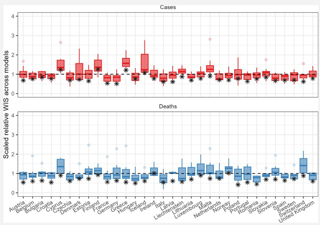
Relative WIS across models against a persistence baseline, 2 weeks ahead, 2021-2022. * = ensemble. Sherratt et al. 2023, eLife.

Aggregated performance varied more with the process being predicted than between forecasters

Data 1 · Hubs, set up to evaluate

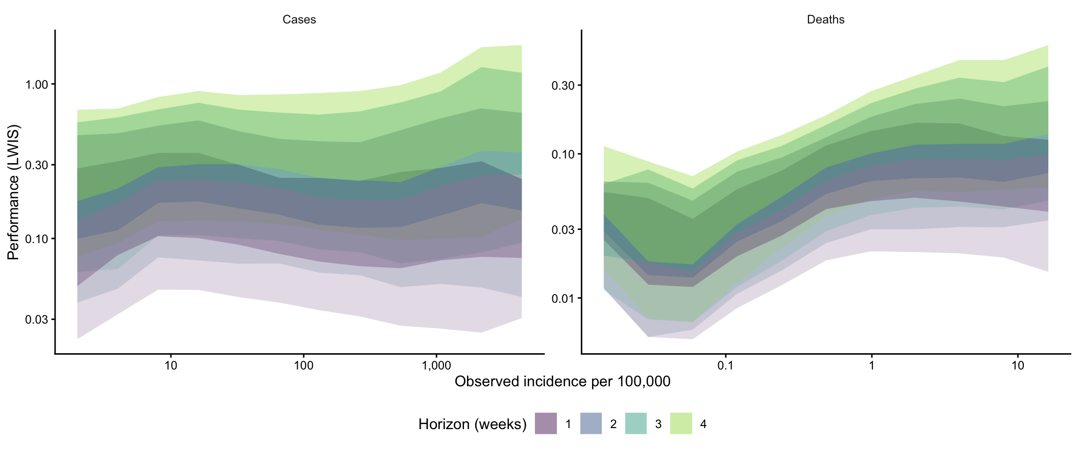
Crude performance shows one consistent thing: the target and the horizon matter. Deaths score better than cases on the log scale, and every outcome gets worse further ahead.

Approaches to controlling variation in comparative forecast evaluation

Theory 2 · Handling confounding

Threat to validity	Approach	Example in forecast evaluation	Limitation
None	Unadjusted comparison	Rank models over all forecasts as submitted	Mixes up the method with the difficulty of the targets each model chose
Confounding, selection	Inclusion criteria	Exclude forecasts without comparable uncertainty	Loses power; narrows the population
Confounding	Matching	Compare forecasters only on targets both submitted	Sparse overlap; holds only for the matched set
Confounding	Stratification	Scores by horizon, location or epidemic phase	Cells sparse with several factors; continuous covariates need binning
Differential population sizes	Indirect standardisation	Relative skill against a baseline available for all targets	Depends on the reference, which changes rankings
Confounding, clustering	Regression adjustment	Partial effect of structure, adjusting for the target	Specification-dependent; estimand informal

Rows run from no control to full adjustment, each borrowed from observational study design.

Participation varied by country, over time, and by model structure

Data 2 · Hubs are sparse

viewof pMethod = Inputs.select(["All structures", ...methodLevels], {label: "Structure"})
viewof pOutcome = Inputs.radio(["Cases", "Deaths"], {value: "Cases", label: "Outcome"})

partT = transpose(participation)
Plot.plot({
  width: 1000, height: 340, marginLeft: 40,
  x: {label: "Week, March 2021 to March 2023", ticks: []},
  y: {label: null},
  color: {type: "sequential", scheme: "viridis", label: "Models forecasting 1 week ahead", legend: true},
  marks: [
    Plot.cell(partT.filter(d => d.Method === pMethod && d.epi_target === pOutcome),
      {x: "forecast_date", y: "Location", fill: "n", inset: 0, tip: true})
  ]
})

One week ahead shown. Every included model forecast all four horizons, so the other horizons look the same. Median participation: 3% of available targets per model.

Click through the structures. Agent-based and judgement cover only a handful of countries and weeks.

Stratification would produce sparse data

Data 2 · Hubs are sparse

viewof strataBy = Inputs.checkbox(varLabels, {value: varLabels, label: "Stratify by"})

sparsityT = transpose(sparsity)
sRow = sparsityT.find(d => d.key === [...strataBy].sort().join("|"))
html`<div class="stats">
  <div><span>${sRow.possible.toLocaleString()}</span>possible strata</div>
  <div><span>${sRow.filled}%</span>contain any forecast</div>
  <div><span>${sRow.median_n.toLocaleString()}</span>median forecasts per filled stratum</div>
  <div><span>${sRow.pct_thin}%</span>of filled strata hold fewer than 5</div>
</div>`

Untick covariates to see how fast the sample thins. Continuous covariates (incidence, horizon) would need binning on top.

Ask the room: which two covariates would you drop first? Try it live. Country and variant phase do the most damage.

Model-based analysis

Theory 3 · Use a regression

Generalised additive mixed model of each forecast’s LWIS (Tweedie, log link). Effects are ratios against the average score: 0.8 is 20% better than average.

Target-generating	Enters as
Outcome (cases, deaths)	Fixed effect
Epidemic trend	Random intercept
Variant phase	Random intercept
Country	Random intercept
Incidence level	Smooth

Forecast-generating	Enters as
Structure × outcome	Random intercept per cell
Single or multi-country	Random intercept
Horizon	Smooth per model
Individual model	Random intercept

Random effects shrink sparse groups towards the average. With 48 models, the effective sample for structure is 48, not 207,973.

Adjusting for the forecasting context alters the interpretation of variation

Data 3 · Results

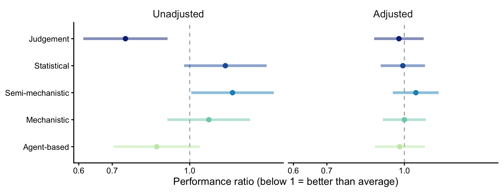
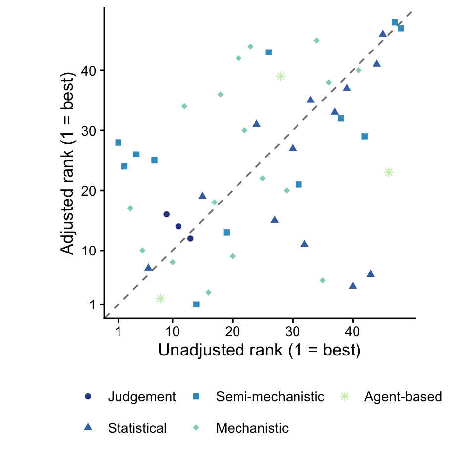
Unadjusted, judgement looks 26% better than average. Adjusted, every structure sits between 0.98 and 1.05, all intervals spanning 1.

Judgement and agent-based are 6 of 48 models and under 5% of forecasts.

Differences between model structures were modified by epidemiological outcome

Data 3 · Results

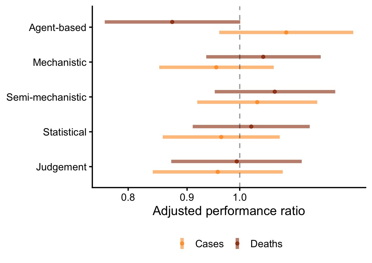
We noted that differences between outcomes largely offset when averaged. An averaged estimate therefore gives close to zero for most structures, whether or not outcome-specific differences exist.

Agent-based, the widest split, rests on 3 models for cases and 2 for deaths. A Gaussian refit reverses the direction for two of five structures.

Wider influences on forecast performance

Data 3 · Results

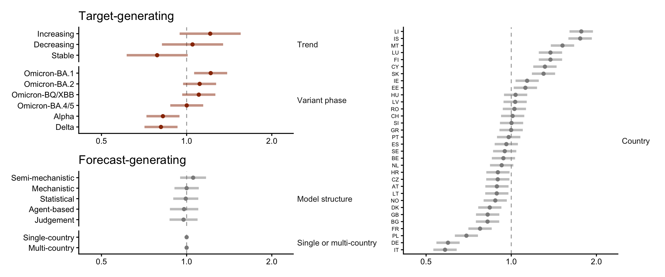
Adjusted performance ratio (95% CI) against the average LWIS, for every categorical term except the 48 individual models. Highlighted: epidemic trend and variant phase. Deaths vs cases is a fixed contrast, ratio 0.35, not shown.

Which models look best depends on how the evaluation is designed

Data 3 · Results

viewof rankHighlight = Inputs.select(["All structures", ...methodLevels], {label: "Highlight"})

ranksT = transpose(ranks)
ranksLong = ranksT.flatMap(d => [
  {...d, stage: "Unadjusted", rank: d.rank_unadjusted},
  {...d, stage: "Adjusted", rank: d.rank_adjusted}
])
Plot.plot({
  width: 520, height: 340,
  x: {type: "point", domain: ["Unadjusted", "Adjusted"], label: null, inset: 40},
  y: {reverse: true, label: "Rank (1 = best)", domain: [1, ranksT.length]},
  color: {domain: methodLevels, range: methodColours},
  marks: [
    Plot.line(ranksLong, {x: "stage", y: "rank", z: "label", stroke: "classification",
      strokeWidth: 2,
      strokeOpacity: d => rankHighlight === "All structures" || d.classification === rankHighlight ? 0.9 : 0.08}),
    Plot.dot(ranksLong, {x: "stage", y: "rank", fill: "classification", r: 4,
      fillOpacity: d => rankHighlight === "All structures" || d.classification === rankHighlight ? 1 : 0.1}),
    Plot.tip(ranksLong, Plot.pointer({x: "stage", y: "rank",
      title: d => `${d.label}\n${d.rank_unadjusted} → ${d.rank_adjusted}`}))
  ]
})

Spearman 0.44. 23 of 48 models move at least 10 places; the furthest moves 37.

Conceptual limitations

Theory 4 · Conceptual limitations

What is a model structure?

Five labels from optional metadata. Raters disagreed on 35%, mostly semi-mechanistic. Methods changed over time and we did not track it.

Impact: misclassification pulls any structure effect towards the null.

Sample

48 models is the effective sample; judgement and agent-based are 6.

Impact: wide intervals for the rare structures; no claim beyond this Hub.

Adjustment

Structure is a property of a model. Horizon is also fitted per model, so it can absorb structure × horizon.

Impact: we estimate a direct effect of structure, after the model’s own quirks.

What could we not see?

Team capacity, experience and time plausibly shape both the choice of structure and the score. We scored against data as of March 2023, not what forecasters saw.

Impact: residual confounding; the estimand stays exploratory.

The choice of evaluation design is not neutral

Theory 4 · Conceptual limitations

To answer “does model structure matter?” from a Hub, we would need:

• Structured metadata: what each model is, and when it changed
• A sampling design: enough independent models of each kind, on shared targets
• A stated estimand: which effect, adjusted for what

Hubs are built to produce a good ensemble, but not to explain individual performance.

Sensitivity analysis: no estimate changed materially

Data 4 · Sensitivity

Check	Structure effect
Natural-scale WIS instead of log	No material change
Raw counts instead of per 100,000	Near-zero impact on scores or fit
Covariate sets (with and without variant phase, outcome)	No material change
Link function	No material change
Gaussian or Gamma instead of Tweedie	By-outcome estimates shift; under Gaussian every interval still spans 1

No specification made any model structure clearly different from the average.

Summary

Theory 1 A score comes from a forecast and a target; unadjusted comparisons mix the two

Data 1 Crude scores mostly track the target and horizon

Theory 2 Designs run from unadjusted to formal; choose by the question

Data 2 Teams pick targets; full stratification leaves 30% of strata filled

Theory 3 Regression uses every forecast, with target and forecaster terms side by side

Data 3 No structure beats average; trend and variant shift scores about 20%; ranks move (ρ 0.44)

Theory 4 Hubs lack the metadata, sampling and estimand this question needs

Data 4 Nothing we tried changed the answer

Built in Quarto from modular section files (report/quarto/_*.qmd), with every number computed from saved fits. This deck reuses the same code.

What next?

1. Next steps: increasing formality with propensity weights for participation, or pooling Hubs (US and Europe; COVID-19, flu, RSV) for more models?
2. If not model structure, what is worth knowing about on each side? (Human judgement, handling of data revisions, update frequency, LLM assistance?)