Sensitivity and comparison analyses
This page continues the main analysis from the one-week-ahead forecast onward: forecast validation, forecast scoring across releases, the reproduction number by release, the outbreak size each data stream implies alone, how the estimate has evolved across releases, comparisons with McCabe et al. and Chamla et al., and the delay and tree-prior sensitivity re-fits. It renders from the same fitted chains as the main analysis, loaded through the shared setup, so no model is re-fit here beyond the frozen re-fits and the optional sensitivity re-fits below.
Load packages, data and fitted chains
# Shared setup: packages, observations, the fit registry and every model fit
# (loaded from the content-addressed cache). See docs/examples/_setup.jl.
using BVDOutbreakSize
include(joinpath(pkgdir(BVDOutbreakSize), "docs", "examples", "_setup.jl"))45Forecast validation
How last week's forecast held up against the data since observed, using the frozen re-fit and one-week projection defined in forecast-versus-frozen evaluation. Only the streams the situation reports are still updating are validated here. A stream that has stopped being reported carries a cumulative total that repeats its last reported value, so there is no observation for the past week to score against. The scoring tables further down withhold such a window for the same reason. The projections for those streams are shown separately below. The frozen fit also conditions on the isolation beds, so the projected bed occupancy is scored against the beds held a week later. The bed validation is weak at a one-week-back freeze. The reported occupancy rate starts only on 9 June, so the capacity has no implied-capacity anchor and rides its random walk back to the freeze date. This widens the projected bed interval. Like the scores further down, the confirmed new-count rows here take out any retrospective harmonisation step the week contained. Such a step reattaches records notified earlier, so it is not something the forecast was predicting. A validation week containing no harmonisation day carries no correction, and the rows then read as the raw window counts. The cumulative rows are scored against the published total, harmonisation included.
Fit one week back and validate the one-week-ahead forecast
# frozen_lastweek and frozen_lastweek_streams are computed in the setup
# block above.
# `obs_recovered` is passed so the frozen fit's forecast carries a
# `recovered_new` column (materialised only when the recovered origin is
# given), letting the recovered stream be scored against the observed count
# below like the other streams.
# The onset grid is the one the FROZEN fit saw, not the live one, so the
# validation forecast carries an `onset reports` row scored on the triangle
# the frozen fit was actually fitted to.
_val_onset_days = frozen_lastweek.o.onset_curve_history.onset_days
_val_grid_start = isempty(_val_onset_days) ? nothing :
                  minimum(_val_onset_days)
_val_grid_end = isnothing(_val_grid_start) ? nothing :
                max(maximum(frozen_lastweek.o.onset_curve_history.report_days),
    _val_grid_start)
validation_forecast = forecast_reported(frozen_lastweek.chn;
    horizon = 7,
    obs_cases = frozen_lastweek.o.reported_cases,
    obs_deaths = frozen_lastweek.o.total_deaths,
    obs_confirmed = frozen_lastweek.o.confirmed_cases,
    obs_confirmed_deaths = frozen_lastweek.o.confirmed_deaths,
    obs_recovered = frozen_lastweek.o.recovered_cases,
    grid_n = frozen_lastweek.o.n,
    onset_grid_start = _val_grid_start, onset_grid_end = _val_grid_end);

# Each frozen individual (single-stream) fit's own one-week-ahead new-count
# forecast at the same cut-off as `frozen_lastweek`, from
# [`forecast_stream`](@ref) (the same per-stream forecaster
# `stream_forecasts.csv` uses), so the validation plots below can show the
# individual fit alongside the joint rather than the joint alone. Recovered
# has no individual fit and is absent here, as it is throughout this report.
# Only the still-reported streams are fitted at the validation cut-off, so
# a stream the situation reports have stopped updating is absent from
# `frozen_lastweek_streams` and carries no individual series here.
function _validation_individual_new(sid, stream::Symbol, obs_field)
    haskey(frozen_lastweek_streams, sid) || return nothing
    f = frozen_lastweek_streams[sid]
    bp = f.o.n - f.o.who_first_sitrep_days
    return Float64.(forecast_stream(f.chn, stream; horizon = 7,
        obs_value = getproperty(f.o, obs_field), n = f.o.n, breakpoint = bp,
        rt_start = 1, rt_walk_start = 1))
end
validation_individual = NamedTuple(
    k => v
for (k, v) in pairs((;
        cases_new = _validation_individual_new(
            "cases", :reported_cases, :reported_cases),
        deaths_new = _validation_individual_new(
            "deaths", :suspected_deaths, :total_deaths),
        confirmed_new = _validation_individual_new(
            "confirmed", :confirmed_cases, :confirmed_cases),
        confirmed_deaths_new = _validation_individual_new(
            "confirmed_deaths", :confirmed_deaths, :confirmed_deaths)))
if !isnothing(v))
# The frozen individual (treatment-only) fit's own bed-occupancy forecast,
# anchored on the beds occupied at ITS OWN cut-off (the frozen fit's own
# `o`, not the current `obs`), matching how the joint frozen forecast is
# itself anchored.
# `nothing` when the beds have stopped being reported, so the treatment fit
# is absent; the bed panel then draws the joint alone.
# A `let` block, not a bare `if`: a top-level `if` shares the script's
# global scope, so its working names would leak into the rest of the page.
validation_individual_isolation = let
    if haskey(frozen_lastweek_streams, "treatment")
        tf = frozen_lastweek_streams["treatment"]
        beds = isempty(tf.o.isolation_history.counts) ? 0.0 :
               Float64(tf.o.isolation_history.counts[end])
        Float64.(forecast_stream(tf.chn, :isolation_beds; horizon = 7,
            obs_value = beds, n = tf.o.n,
            breakpoint = tf.o.n - tf.o.who_first_sitrep_days,
            rt_start = 1, rt_walk_start = 1))
    else
        nothing
    end
end

# The observed beds at the current cut-off (the forecast target), so the
# frozen-fit bed forecast is scored against what the beds actually held.
# Held back once the beds stop being reported, since the last count would
# then be carried forward rather than observed at the target date.
_obs_beds = stream_reporting(obs, :isolation_beds) ?
            obs.isolation_history.counts[end] : missing
# Same observed/baseline keying as the plot below, so the table covers every
# fitted count stream (cumulative and new-count rows) plus the bed level.
# A harmonisation-break day between the frozen cut-off and the current one
# puts records into the confirmed cumulative that were never notified in that
# week, so the new-count truth carries a step the forecast was never
# predicting. Take it out, the same correction `score_releases.jl` applies.
# Grid days are relative to a seeding date fixed by the genetic tmrca, so the
# frozen fit's own `n` and the current `obs.n` index the same grid.
validation_breaks = (
    confirmed_cum = confirmed_break_correction(
        obs, frozen_lastweek.o.n, obs.n),
    confirmed_deaths_cum = confirmed_break_correction(
        obs, frozen_lastweek.o.n, obs.n; deaths = true))

# Observed cumulative at the target date per stream, keyed by the forecast's
# cumulative column; `baseline` is each stream's origin cumulative (the
# frozen cut-off), so the new count is scored against observed minus origin,
# less any harmonisation the window carries (see `validation_breaks`). Both
# the table and the plot below take the still-reported streams
# (`reporting_cum_cols`, from the setup block): a stream the situation
# reports have stopped updating has an origin and a target reading the same
# repeated total, so its cumulative truth is stale and its new-count truth is
# a guaranteed zero.
validation_observed = (cases_cum = obs.reported_cases,
    deaths_cum = obs.total_deaths,
    confirmed_cum = obs.confirmed_cases,
    confirmed_deaths_cum = obs.confirmed_deaths,
    recovered_cum = obs.recovered_cases)
validation_baseline = (cases_cum = frozen_lastweek.o.reported_cases,
    deaths_cum = frozen_lastweek.o.total_deaths,
    confirmed_cum = frozen_lastweek.o.confirmed_cases,
    confirmed_deaths_cum = frozen_lastweek.o.confirmed_deaths,
    recovered_cum = frozen_lastweek.o.recovered_cases)

validation_table = forecast_vs_truth(validation_forecast;
    observed = keep_streams(validation_observed, reporting_cum_cols),
    baseline = keep_streams(validation_baseline, reporting_cum_cols),
    breaks = validation_breaks,
    isolation = _obs_beds);
Forecast-versus-observed validation table
# `MarkdownTable` rather than a bare table expression: a DataFrame is
# `text/html`-showable, Literate prefers that mime, and the `@raw html`
# block it writes crosses Documenter's raw-block regex limit once the
# table grows. `MarkdownTable` is markdown-showable and not
# html-showable, so the table goes out as an ordinary markdown table
# rather than a fixed-width block of printed output. See its docstring
# for the mechanism. The same treatment is applied to every DataFrame
# display in this file and in `analysis.jl`.| Stream | Quantity | Observed | Lower 90% | Lower 60% | Lower 30% | Upper 30% | Upper 60% | Upper 90% | Within 90% PI |
|---|---|---|---|---|---|---|---|---|---|
| DRC confirmed cases | cumulative by T+7 | 6686 | 6560 | 6648 | 6712 | 6827 | 6901 | 7050 | yes |
| DRC confirmed cases | new this week | 586 | 460 | 548 | 612 | 727 | 801 | 950 | yes |
| DRC confirmed deaths | cumulative by T+7 | 3226 | 3176 | 3212 | 3238 | 3282 | 3308 | 3367 | yes |
| DRC confirmed deaths | new this week | 276 | 226 | 262 | 288 | 332 | 358 | 417 | yes |
| DRC recovered | cumulative by T+7 | 1563 | 1559 | 1697 | 1761 | 1871 | 1950 | 2113 | yes |
| DRC recovered | new this week | 180 | 176 | 314 | 378 | 488 | 567 | 730 | yes |
| DRC isolation beds | occupancy at T+7 | 819 | 618 | 719 | 772 | 857 | 923 | 1038 | yes |
The observation panels histogram the one-week-ahead forecast made from the frozen fit: a cumulative and a new-count panel for each still-reported count stream the forecast carries. The 90% predictive interval is shaded, and the count observed by the current cut-off is a dashed black rule. Each stream draws only when the forecast carries its column and the observation covers the target date, so a fit observing fewer streams shows fewer panels. Where a stream has its own individual (single-stream) fit, that fit's forecast from the same frozen cut-off is overlaid as a dotted density alongside the joint's histogram. Recovered has no individual fit and draws the joint alone.
Forecast-versus-observed plot
validation_fig = plot_forecast_vs_truth(validation_forecast;
    observed = keep_streams(validation_observed, reporting_cum_cols),
    baseline = keep_streams(validation_baseline, reporting_cum_cols),
    breaks = validation_breaks,
    individual = keep_streams(validation_individual, reporting_cum_cols));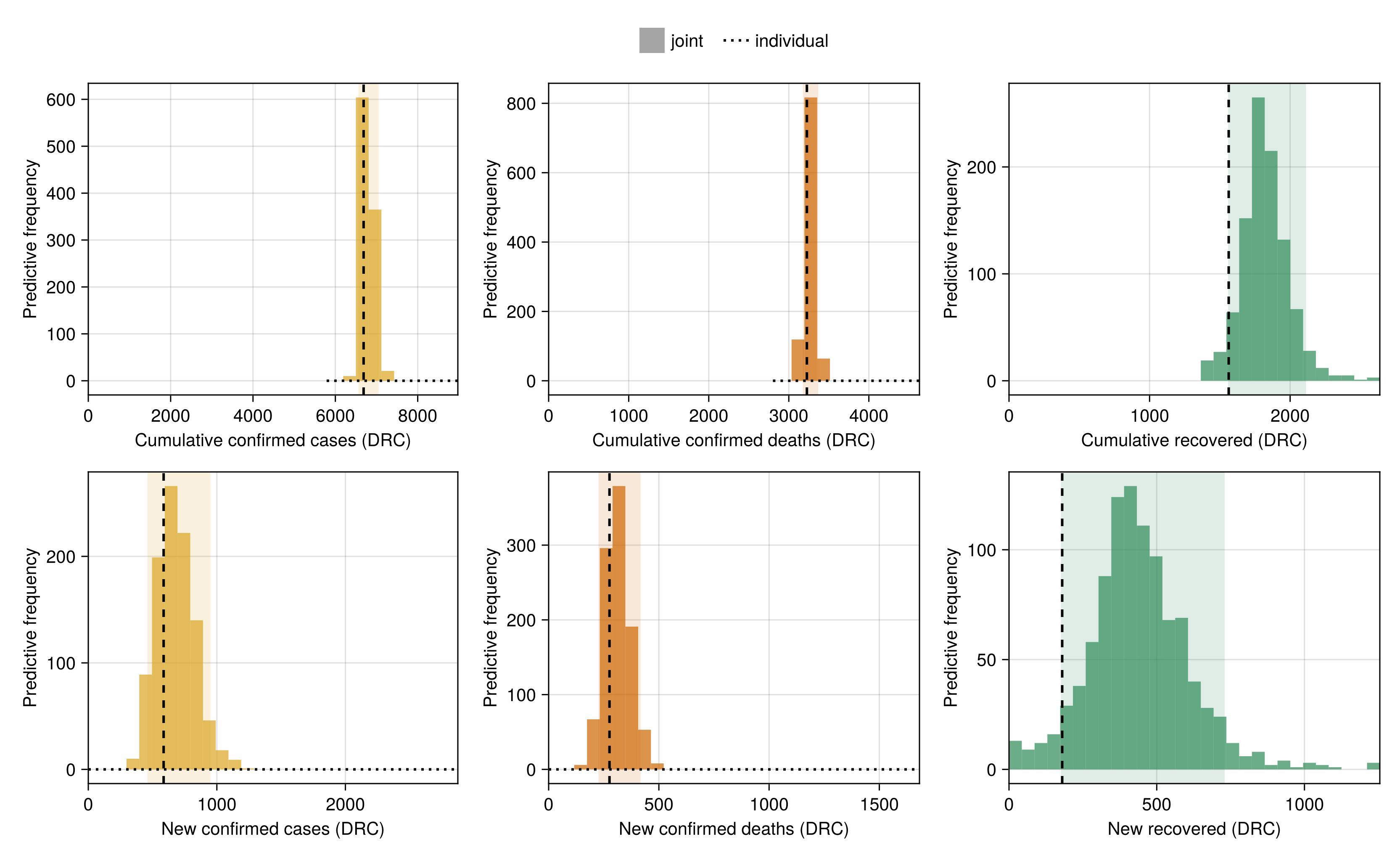
The bed panel scores last week's projected occupancy against the beds occupied now (the dashed rule), with the individual (treatment-only) fit's own projection overlaid as a dotted density alongside the joint.
Bed forecast-versus-observed plot
validation_beds_fig = plot_forecast_beds_vs_truth(validation_forecast;
    isolation = _obs_beds, individual = validation_individual_isolation);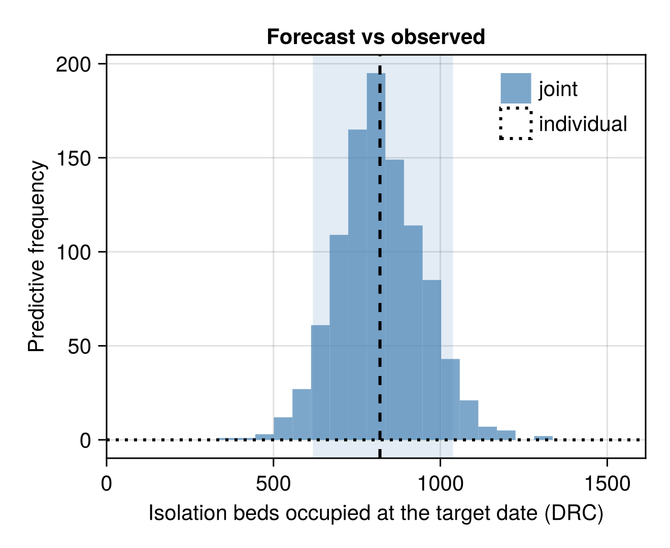
The latent quantities are not observed, so they are scored distribution against distribution: what the frozen fit forecast for the past week's new infections, onsets and deaths against what the current fit now estimates for the same window.
Forecast-versus-now latent plot
# Current fit's draws of the new latent counts over the past week, the last
# seven days of each cumulative-trajectory deterministic.
function _now_new(chn, key)
    mat = chn[key]
    trajs = [collect(v) for v in vec(collect(mat))]
    return Float64[t[end] - t[max(1, length(t) - 7)] for t in trajs]
end
now_latent = (;
    infections_new = _now_new(chn_joint, :cumulative_infections),
    onsets_new = _now_new(chn_joint, :cumulative_onsets),
    deaths_latent_new = _now_new(chn_joint, :cumulative_expected_deaths))

validation_latent_fig = plot_forecast_vs_truth_latent(
    validation_forecast; now = now_latent);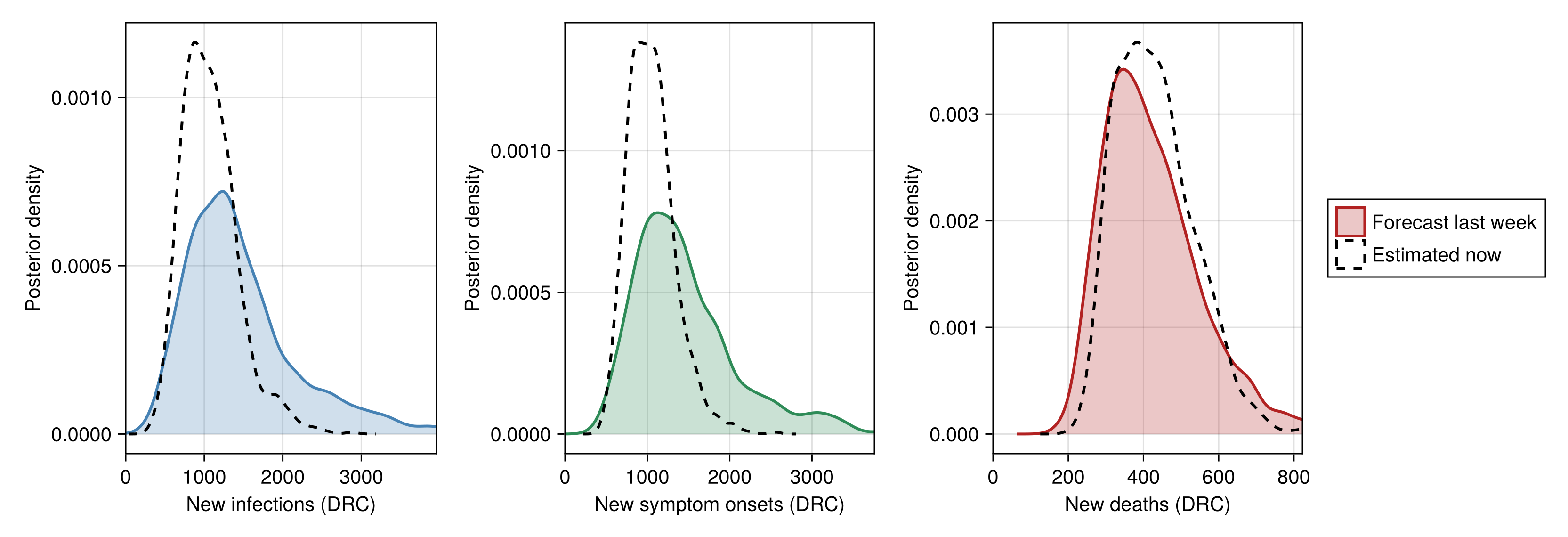
Streams no longer reported
The situation reports have stopped updating some of the streams the model fits, listed with the date each was last reported below. The panels show what the frozen fit projected for those streams over the same week, without an observed rule, since the count they would be scored against has not moved since the stream stopped. These are the model's projections rather than a validation of them.
Forecast for the streams no longer reported
# The last-reported date per stopped stream, and the frozen fit's own
# projection for them. `plot_forecast` draws a panel per new-count column
# the frame carries, so passing the stopped streams' columns alone gives the
# projection without the fabricated truth rule the validation figure would
# otherwise draw against a repeated total.
validation_stopped_streams = let s = stream_report_status(obs),
    ids = [stream_id(c) for c in stopped_cum_cols]

    keep = [r.stream in ids for r in eachrow(s)]
    DataFrame("Stream" => s[keep, :label],
        "Last reported" => s[keep, :last_date])
end
_stopped_new_cols = [c
                     for c in new_cols(stopped_cum_cols)
                     if c in propertynames(validation_forecast)]
validation_stopped_fig = plot_forecast(
validation_forecast[!, _stopped_new_cols]);# See the comment above `validation_table`'s display for why this wraps
# the table in `MarkdownTable` instead of showing it directly.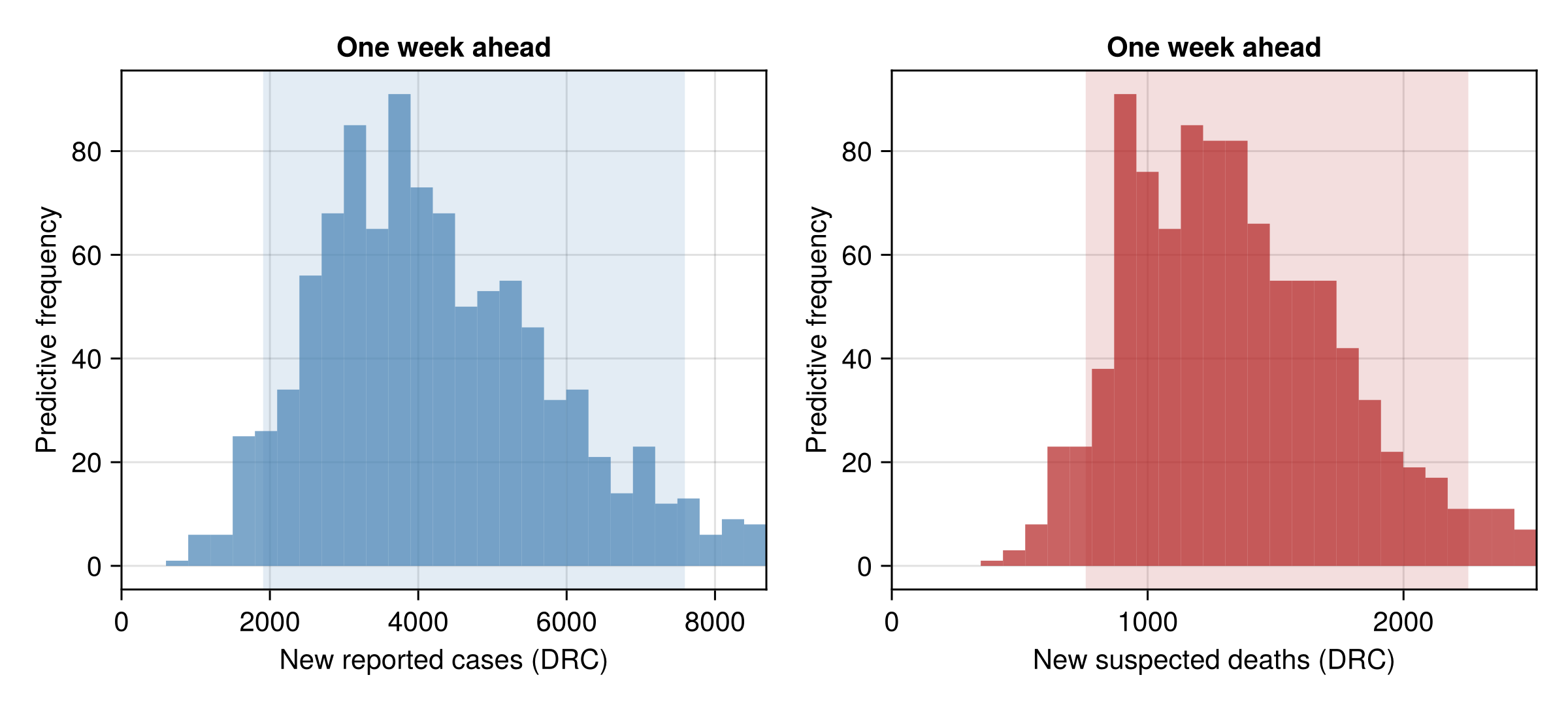
Forecast scoring across releases
Every release's saved one- to four-week-ahead forecast is scored against the data observed since, against a persistence baseline and, where one exists, the stream's own individual fit as well as the joint. The tables in this section are the joint model's, one row per stream. Each stream's individual fit is scored the same way and tabulated in Individual fits against the baseline below, so a fit appears in one table rather than two. See forecast scoring against a persistence baseline for how the scores, the relative skill and the baseline are built. Recovered has no individual fit of its own, so its comparison is the baseline against the joint only. Reported cases and suspected deaths stopped being updated by the situation reports partway through the outbreak, and exports' confirmed-detection series is anchored to an earlier cut-off. Exports therefore contributes no scored forecast, and reported cases and suspected deaths each rest on exactly one matched forecast, a single window rather than a settled sample.
Only a minority of the daily releases examined contribute a row to the table below, each a reconstruction of an earlier model version rather than the current fit. The table below is therefore not a verdict on the current fit. One reconstruction is dropped from scoring entirely: its chain forecasts a near-zero median at every horizon and stream, with the upper predictive tail occasionally reaching five- and six-digit values. This is the signature of a chain that failed to sample properly rather than a genuine forecast, so the scoring script flags and excludes it. Only the newest few releases carry the current model's own individual-stream forecasts, and the backfilled reconstructions carry none at all. The comparison against each stream's individual fit therefore rests on those releases alone, filling in one horizon at a time as their targets resolve. Every row also rests on one to a handful of matched forecasts, shown as its own count rather than rounded away. A ratio here should therefore be read as an early signal rather than a settled result.
The symptom-onset stream is scored on the new reported count each vintage adds rather than on its level, because every vintage rereads the whole figure. Its printed total therefore moves with the scan error as well as with late reporting. It appears only from the release that first carried it. Its intervals are dominated by that scan error rather than by epidemic uncertainty, so read its skill against the baseline rather than its coverage.
Load and summarise the cross-release forecast scores
# scripts/score_releases.jl writes these after the fits. The committed files
# are header-only until a release carries the asset, so the common path
# reads a real file to a zero-row frame; the typed `schema` is the fallback
# for a file that is absent entirely, since CSV.read throws on a missing
# path and would take the whole docs build with it.
function _release_data(name, schema::NamedTuple)
    path = joinpath(pkgdir(BVDOutbreakSize), "data", name)
    isfile(path) && return CSV.read(path, DataFrame)
    return DataFrame([k => T[] for (k, T) in pairs(schema)])
end

forecast_scores_df = _release_data("forecast_scores.csv",
    (; release = String, made_date = Date, stream = String, horizon = Int,
        target_date = Date, fit = String, crps = Float64,
        log_crps = Float64, dispersion = Float64, overprediction = Float64,
        underprediction = Float64, coverage_50 = Float64,
        coverage_90 = Float64,
        bias = Float64, n_samples = Int,
        log_rel_to_baseline = Float64))
forecast_overlay_df = _release_data("forecast_overlay.csv",
    (; release = String, made_date = Date, stream = String, horizon = Int,
        target_date = Date, fit = String, observed = Float64,
        median = Float64, lo30 = Float64, hi30 = Float64, lo60 = Float64,
        hi60 = Float64, lo90 = Float64, hi90 = Float64))
# One row per (stream, fit) pooled over every horizon and release. The
# by-horizon and by-release detail tables carry the same columns at a finer
# grain (see src/scoring.jl). Every fit is kept here, since the
# relative-skill figure below compares the roles against each other. The
# tables rendered in this section select the joint role, and the individual
# fits are tabulated in their own section.
forecast_score_overview_table = forecast_score_overview(forecast_scores_df)
forecast_score_by_horizon_table = forecast_score_by_horizon(forecast_scores_df)
forecast_score_by_release_table = forecast_score_by_release(forecast_scores_df)

joint_score_overview_table = select_fit_role(
    forecast_score_overview_table, "joint")
joint_score_by_horizon_table = select_fit_role(
    forecast_score_by_horizon_table, "joint")
# The trailing `;` on this last assignment matters: without it, this whole
# setup chunk's last statement (the DataFrame it assigns) is Literate's
# implicitly displayed "result" for the chunk, on top of the deliberate
# display further down -- and a bare DataFrame is html-showable, so it
# goes out as a second, undisplayed-in-source `@raw html` block that (for
# a table this size) can itself hit the PCRE limit described above.
joint_score_by_release_table = select_fit_role(
    forecast_score_by_release_table, "joint");
The headline pools every horizon and release into one row per stream for the joint model: the mean CRPS and its decomposition, coverage, bias, and the relative skill against the persistence baseline, on both the natural and the log scale. Each row also carries relative skill against the stream's own individual fit where one exists. Column definitions are in forecast scoring against a persistence baseline.
| stream | fit | n | crps | rel_to_baseline | log_crps | log_rel_to_baseline | rel_to_individual | log_rel_to_individual | dispersion | overprediction | underprediction | coverage_50 | coverage_90 | bias |
|---|---|---|---|---|---|---|---|---|---|---|---|---|---|---|
| confirmed cases | joint | 70 | 1159.7 | 7.03 | 0.233 | 1.79 | 0.8 | 0.75 | 1097.36 | 61.76 | 0.58 | 0.84 | 1 | 0.21 |
| confirmed deaths | joint | 68 | 1226.26 | 10.82 | 0.581 | 3.2 | 0.92 | 1.66 | 1099.46 | 5.62 | 121.18 | 0.38 | 0.99 | -0.46 |
| isolation beds | joint | 65 | 73.63 | 1.36 | 0.096 | 1.3 | 0.88 | 0.69 | 44.58 | 21.96 | 7.1 | 0.6 | 0.94 | 0.19 |
| onset reports | joint | 25 | 166.5 | 0.89 | 0.467 | 0.68 | 0.81 | 0.89 | 77.46 | 64.16 | 24.89 | 0.4 | 0.96 | 0.19 |
| recovered | joint | 11 | 139.4 | 1.68 | 0.376 | 1.09 | missing | missing | 120.02 | 6.31 | 13.07 | 1 | 1 | -0.18 |
The same relative skill against the baseline, by horizon: one panel per stream, one series per fit role, on a log-scaled skill axis with the reference line at one. This is the one place the two roles are drawn against each other, so it carries each stream's individual fit alongside the joint. A fit that beats the baseline on average but not at every cut-off is visible as a series that crosses the line rather than sitting under it throughout.
forecast_relative_skill_fig = plot_forecast_relative_skill(
    forecast_score_by_horizon_table);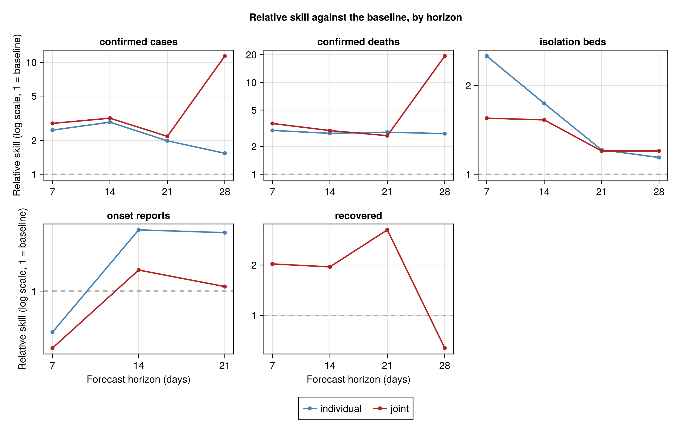
The same columns as a table for the joint model, broken out by horizon, and again broken out by release and averaged across horizons, are behind the two dropdowns below.
Scores by horizon
| stream | horizon | fit | n | crps | rel_to_baseline | log_crps | log_rel_to_baseline | rel_to_individual | log_rel_to_individual | dispersion | overprediction | underprediction | coverage_50 | coverage_90 | bias |
|---|---|---|---|---|---|---|---|---|---|---|---|---|---|---|---|
| confirmed cases | 7 | joint | 22 | 105.01 | 2.85 | 0.235 | 3.07 | 0.81 | 0.72 | 82.07 | 22.07 | 0.87 | 0.77 | 1 | 0.24 |
| confirmed cases | 14 | joint | 19 | 234.99 | 3.17 | 0.237 | 2.97 | 0.8 | 0.74 | 189.34 | 44.95 | 0.7 | 0.89 | 1 | 0.18 |
| confirmed cases | 21 | joint | 16 | 471.59 | 2.18 | 0.219 | 1.33 | 0.77 | 0.75 | 386.85 | 84.34 | 0.4 | 0.88 | 1 | 0.18 |
| confirmed cases | 28 | joint | 13 | 5142.95 | 11.38 | 0.238 | 0.96 | 0.82 | 0.81 | 5017.12 | 125.69 | 0.14 | 0.85 | 1 | 0.22 |
| confirmed deaths | 7 | joint | 22 | 83.75 | 3.57 | 0.594 | 5.75 | 1.15 | 1.32 | 33.34 | 0.65 | 49.76 | 0.45 | 0.95 | -0.43 |
| confirmed deaths | 14 | joint | 18 | 203.51 | 2.99 | 0.569 | 3.86 | 1.25 | 1.95 | 88.04 | 1.93 | 113.54 | 0.33 | 1 | -0.49 |
| confirmed deaths | 21 | joint | 15 | 393.79 | 2.63 | 0.588 | 2.7 | 1.01 | 1.95 | 211.54 | 7.22 | 175.04 | 0.2 | 1 | -0.5 |
| confirmed deaths | 28 | joint | 13 | 5536.39 | 19.35 | 0.566 | 1.77 | 0.7 | 1.64 | 5328.64 | 17.29 | 190.46 | 0.54 | 1 | -0.43 |
| isolation beds | 7 | joint | 20 | 64.53 | 1.55 | 0.083 | 1.44 | 0.68 | 0.52 | 31.27 | 26.25 | 7.01 | 0.45 | 0.95 | 0.29 |
| isolation beds | 14 | joint | 17 | 74.39 | 1.53 | 0.093 | 1.39 | 0.93 | 0.69 | 44.87 | 24.04 | 5.47 | 0.59 | 0.94 | 0.22 |
| isolation beds | 21 | joint | 15 | 78.48 | 1.2 | 0.102 | 1.15 | 1.01 | 0.81 | 51.79 | 18.13 | 8.57 | 0.73 | 0.93 | 0.12 |
| isolation beds | 28 | joint | 13 | 81.05 | 1.2 | 0.114 | 1.25 | 1.03 | 0.91 | 56.34 | 17.04 | 7.66 | 0.69 | 0.92 | 0.09 |
| onset reports | 7 | joint | 11 | 121.83 | 0.61 | 0.786 | 0.64 | 0.88 | 0.96 | 55.6 | 48.71 | 17.52 | 0.27 | 1 | 0.18 |
| onset reports | 14 | joint | 8 | 212.15 | 1.2 | 0.266 | 0.91 | 0.7 | 0.72 | 78.1 | 85.7 | 48.35 | 0.25 | 0.88 | 0.26 |
| onset reports | 21 | joint | 6 | 187.54 | 1.04 | 0.149 | 0.73 | 0.63 | 0.63 | 116.67 | 63.75 | 7.12 | 0.83 | 1 | 0.12 |
| recovered | 7 | joint | 3 | 26.96 | 2.03 | 0.319 | 1.67 | missing | missing | 20.93 | 1.28 | 4.76 | 1 | 1 | -0.18 |
| recovered | 14 | joint | 3 | 89.7 | 1.95 | 0.393 | 1.45 | missing | missing | 68.01 | 5.81 | 15.87 | 1 | 1 | -0.23 |
| recovered | 21 | joint | 3 | 297.16 | 3.24 | 0.422 | 1.15 | missing | missing | 269.9 | 16.05 | 11.2 | 1 | 1 | -0.09 |
| recovered | 28 | joint | 2 | 145.99 | 0.64 | 0.367 | 0.56 | missing | missing | 121.86 | 0 | 24.13 | 1 | 1 | -0.26 |
Scores by release
| made_date | stream | fit | n | crps | rel_to_baseline | log_crps | log_rel_to_baseline | rel_to_individual | log_rel_to_individual | dispersion | overprediction | underprediction | coverage_50 | coverage_90 | bias |
|---|---|---|---|---|---|---|---|---|---|---|---|---|---|---|---|
| 2026-06-07 | confirmed cases | joint | 2 | 363.91 | 14.18 | 0.913 | 11.98 | missing | missing | 341.06 | 22.86 | 0 | 1 | 1 | 0.17 |
| 2026-06-10 | confirmed cases | joint | 3 | 534.87 | 6.69 | 0.791 | 4.97 | missing | missing | 435.67 | 99.2 | 0 | 1 | 1 | 0.27 |
| 2026-07-01 | confirmed cases | joint | 4 | 15862.78 | 74.74 | 0.583 | 2.84 | missing | missing | 15377.31 | 485.47 | 0 | 0 | 1 | 0.66 |
| 2026-07-06 | confirmed cases | joint | 4 | 421.28 | 1.31 | 0.269 | 0.95 | missing | missing | 311.85 | 109.43 | 0 | 0.5 | 1 | 0.49 |
| 2026-07-08 | confirmed cases | joint | 4 | 390.98 | 1.23 | 0.253 | 0.97 | missing | missing | 239.5 | 151.47 | 0 | 0.25 | 1 | 0.52 |
| 2026-07-23 | confirmed cases | joint | 4 | 335.57 | 0.86 | 0.169 | 0.66 | 1.02 | 0.82 | 299.27 | 35.68 | 0.62 | 1 | 1 | 0.13 |
| 2026-07-25 | confirmed cases | joint | 4 | 222.5 | 0.98 | 0.134 | 0.99 | 0.64 | 0.63 | 218.04 | 4.46 | 0 | 1 | 1 | 0.07 |
| 2026-07-26 | confirmed cases | joint | 4 | 235.69 | 1.07 | 0.141 | 1.06 | 0.79 | 0.67 | 229.65 | 5.68 | 0.36 | 1 | 1 | 0.06 |
| 2026-07-27 | confirmed cases | joint | 4 | 247.97 | 1.22 | 0.142 | 1.07 | 0.93 | 0.83 | 240.08 | 7.88 | 0 | 1 | 1 | 0.11 |
| 2026-07-31 | confirmed cases | joint | 4 | 259.64 | 1.85 | 0.149 | 1.69 | 0.64 | 0.68 | 235.73 | 23.76 | 0.15 | 1 | 1 | 0.13 |
| 2026-08-01 | confirmed cases | joint | 4 | 231.26 | 1.97 | 0.139 | 1.99 | 0.69 | 0.66 | 226.84 | 4.31 | 0.11 | 1 | 1 | 0.05 |
| 2026-08-02 | confirmed cases | joint | 4 | 278.45 | 2.12 | 0.145 | 1.75 | 0.94 | 0.85 | 263.77 | 14.68 | 0 | 1 | 1 | 0.14 |
| 2026-08-03 | confirmed cases | joint | 4 | 247.58 | 1.29 | 0.14 | 0.96 | 0.85 | 0.8 | 237.88 | 9.7 | 0 | 1 | 1 | 0.08 |
| 2026-08-04 | confirmed cases | joint | 4 | 221.56 | 2.43 | 0.133 | 2.39 | 0.63 | 0.69 | 220.7 | 0.86 | 0 | 1 | 1 | 0.03 |
| 2026-08-07 | confirmed cases | joint | 4 | 213.54 | 2.39 | 0.14 | 2.01 | 0.69 | 0.73 | 209.76 | 0 | 3.78 | 1 | 1 | -0.09 |
| 2026-08-11 | confirmed cases | joint | 3 | 144.14 | 3.41 | 0.13 | 3.34 | 0.61 | 0.71 | 137.28 | 0 | 6.86 | 1 | 1 | -0.15 |
| 2026-08-15 | confirmed cases | joint | 3 | 277.43 | 5.28 | 0.183 | 3.47 | 1.28 | 0.9 | 200.14 | 77.29 | 0 | 1 | 1 | 0.38 |
| 2026-08-17 | confirmed cases | joint | 2 | 202.19 | 2.31 | 0.187 | 1.84 | 1.4 | 0.89 | 125.12 | 77.07 | 0 | 1 | 1 | 0.4 |
| 2026-08-22 | confirmed cases | joint | 2 | 157.12 | 2.86 | 0.161 | 2.63 | 0.98 | 0.84 | 110.93 | 46.2 | 0 | 1 | 1 | 0.44 |
| 2026-08-24 | confirmed cases | joint | 1 | 77.26 | 3.26 | 0.127 | 2.92 | 0.87 | 0.82 | 33.95 | 43.31 | 0 | 0 | 1 | 0.63 |
| 2026-08-25 | confirmed cases | joint | 1 | 74.23 | 2.9 | 0.121 | 2.38 | 0.82 | 0.77 | 33.62 | 40.61 | 0 | 0 | 1 | 0.64 |
| 2026-08-30 | confirmed cases | joint | 1 | 36.49 | 0.84 | 0.058 | 0.72 | 0.41 | 0.42 | 32.57 | 3.92 | 0 | 1 | 1 | 0.2 |
| 2026-06-07 | confirmed deaths | joint | 1 | 41.49 | 1.87 | 0.903 | 2.55 | missing | missing | 36.94 | 0 | 4.55 | 1 | 1 | -0.2 |
| 2026-06-10 | confirmed deaths | joint | 2 | 64.93 | 2.27 | 0.735 | 3.05 | missing | missing | 62.7 | 0.99 | 1.24 | 1 | 1 | -0.03 |
| 2026-07-01 | confirmed deaths | joint | 4 | 17196 | 80.45 | 0.549 | 1.21 | missing | missing | 17103.11 | 92.89 | 0 | 1 | 1 | 0.28 |
| 2026-07-06 | confirmed deaths | joint | 4 | 197.2 | 0.89 | 0.871 | 2.29 | missing | missing | 110.35 | 0 | 86.85 | 0.25 | 1 | -0.49 |
| 2026-07-08 | confirmed deaths | joint | 4 | 177.59 | 0.78 | 0.713 | 1.84 | missing | missing | 84.29 | 0 | 93.3 | 0.25 | 1 | -0.61 |
| 2026-07-23 | confirmed deaths | joint | 4 | 271.49 | 1.67 | 0.484 | 2.45 | 0.39 | 1.08 | 172.61 | 0 | 98.88 | 1 | 1 | -0.45 |
| 2026-07-25 | confirmed deaths | joint | 4 | 241.83 | 1.98 | 0.504 | 3.41 | 1.02 | 2.15 | 106.46 | 0 | 135.37 | 0 | 1 | -0.57 |
| 2026-07-26 | confirmed deaths | joint | 4 | 268.46 | 2.31 | 0.554 | 4.16 | 1.05 | 2.17 | 101.59 | 0 | 166.87 | 0 | 1 | -0.64 |
| 2026-07-27 | confirmed deaths | joint | 4 | 249.47 | 2.29 | 0.534 | 3.99 | 0.8 | 2.12 | 109.3 | 0 | 140.17 | 0 | 1 | -0.59 |
| 2026-07-31 | confirmed deaths | joint | 4 | 274.55 | 2.31 | 0.56 | 3.96 | 0.88 | 1.94 | 108.79 | 0 | 165.76 | 0.25 | 1 | -0.58 |
| 2026-08-01 | confirmed deaths | joint | 4 | 313.48 | 2.69 | 0.683 | 4.66 | 1.12 | 2.7 | 94.48 | 0 | 219.01 | 0 | 1 | -0.68 |
| 2026-08-02 | confirmed deaths | joint | 4 | 258.17 | 2.85 | 0.507 | 4.38 | 1.01 | 1.83 | 128.19 | 0 | 129.98 | 0.25 | 1 | -0.53 |
| 2026-08-03 | confirmed deaths | joint | 4 | 268.89 | 1.96 | 0.58 | 2.91 | 1.2 | 2.37 | 123.56 | 0 | 145.33 | 0.25 | 1 | -0.55 |
| 2026-08-04 | confirmed deaths | joint | 4 | 298.06 | 3.91 | 0.656 | 7.33 | 1.2 | 2.32 | 93.54 | 0 | 204.52 | 0 | 1 | -0.67 |
| 2026-08-07 | confirmed deaths | joint | 4 | 366.29 | 4.84 | 0.88 | 8.05 | 1.58 | 2.71 | 76.06 | 0 | 290.23 | 0 | 0.75 | -0.79 |
| 2026-08-11 | confirmed deaths | joint | 3 | 256.46 | 12.09 | 0.821 | 21.35 | 1.54 | 2.5 | 69.1 | 0 | 187.36 | 0 | 1 | -0.75 |
| 2026-08-15 | confirmed deaths | joint | 3 | 154.31 | 3.71 | 0.321 | 4.39 | 0.91 | 0.97 | 128.64 | 0 | 25.67 | 1 | 1 | -0.28 |
| 2026-08-17 | confirmed deaths | joint | 2 | 105.06 | 2.11 | 0.307 | 2.72 | 0.97 | 1.13 | 83.42 | 0 | 21.64 | 1 | 1 | -0.3 |
| 2026-08-22 | confirmed deaths | joint | 2 | 97.18 | 1.33 | 0.303 | 2.11 | 0.74 | 0.63 | 74.43 | 0 | 22.75 | 1 | 1 | -0.3 |
| 2026-08-24 | confirmed deaths | joint | 1 | 17.41 | 1.57 | 0.055 | 1.49 | 0.18 | 0.1 | 15 | 2.41 | 0 | 1 | 1 | 0.22 |
| 2026-08-25 | confirmed deaths | joint | 1 | 14.89 | 0.92 | 0.049 | 0.82 | 0.14 | 0.06 | 13.83 | 1.06 | 0 | 1 | 1 | 0.16 |
| 2026-08-30 | confirmed deaths | joint | 1 | 19.28 | 1.93 | 0.065 | 1.76 | 0.18 | 0.07 | 14.16 | 5.12 | 0 | 1 | 1 | 0.29 |
| 2026-07-01 | isolation beds | joint | 4 | 90.19 | 1.48 | 0.138 | 1.52 | missing | missing | 13.48 | 0 | 76.71 | 0 | 0 | -0.99 |
| 2026-07-06 | isolation beds | joint | 4 | 42.87 | 0.62 | 0.066 | 0.64 | missing | missing | 21.07 | 0 | 21.8 | 0 | 1 | -0.64 |
| 2026-07-08 | isolation beds | joint | 4 | 54.75 | 1.54 | 0.073 | 1.54 | missing | missing | 11.67 | 43.08 | 0 | 0 | 1 | 0.8 |
| 2026-07-23 | isolation beds | joint | 4 | 80.06 | 2.72 | 0.101 | 2.63 | 1.44 | 1.14 | 29.39 | 50.67 | 0 | 0 | 1 | 0.58 |
| 2026-07-25 | isolation beds | joint | 4 | 80.84 | 2.19 | 0.105 | 2.16 | 1.56 | 1.28 | 32.65 | 48.19 | 0 | 0.5 | 1 | 0.53 |
| 2026-07-26 | isolation beds | joint | 4 | 73.83 | 1.97 | 0.097 | 1.9 | 1.2 | 0.96 | 36.96 | 36.87 | 0 | 0.5 | 1 | 0.46 |
| 2026-07-27 | isolation beds | joint | 4 | 71.58 | 2.47 | 0.093 | 2.35 | 1.2 | 0.95 | 39.52 | 32.06 | 0 | 0.5 | 1 | 0.44 |
| 2026-07-31 | isolation beds | joint | 4 | 71.05 | 1.68 | 0.088 | 1.63 | 0.86 | 0.67 | 51.69 | 19.36 | 0 | 0.75 | 1 | 0.34 |
| 2026-08-01 | isolation beds | joint | 4 | 72 | 1.12 | 0.094 | 1.09 | 0.81 | 0.61 | 64.51 | 7.48 | 0.02 | 1 | 1 | 0.18 |
| 2026-08-02 | isolation beds | joint | 4 | 83.69 | 1.63 | 0.102 | 1.47 | 0.99 | 0.72 | 52.67 | 31.02 | 0 | 0.75 | 1 | 0.39 |
| 2026-08-03 | isolation beds | joint | 4 | 78.83 | 1.85 | 0.099 | 1.72 | 0.99 | 0.74 | 60.42 | 18.41 | 0 | 1 | 1 | 0.3 |
| 2026-08-04 | isolation beds | joint | 4 | 100.74 | 1.43 | 0.137 | 1.36 | 1.16 | 0.98 | 63.47 | 37.28 | 0 | 0.75 | 1 | 0.38 |
| 2026-08-07 | isolation beds | joint | 4 | 83.81 | 1.44 | 0.122 | 1.61 | 0.8 | 0.71 | 69.03 | 0 | 14.78 | 1 | 1 | -0.24 |
| 2026-08-11 | isolation beds | joint | 3 | 64.56 | 0.39 | 0.091 | 0.38 | 0.62 | 0.52 | 61.88 | 0 | 2.68 | 1 | 1 | -0.09 |
| 2026-08-15 | isolation beds | joint | 3 | 73.18 | 0.96 | 0.082 | 0.85 | 0.59 | 0.42 | 64.93 | 8.25 | 0 | 1 | 1 | 0.17 |
| 2026-08-17 | isolation beds | joint | 2 | 73.47 | 1.56 | 0.083 | 1.33 | 0.75 | 0.52 | 57.83 | 15.64 | 0 | 1 | 1 | 0.32 |
| 2026-08-22 | isolation beds | joint | 2 | 63.1 | 1.56 | 0.067 | 1.38 | 0.44 | 0.3 | 52.81 | 10.29 | 0 | 1 | 1 | 0.24 |
| 2026-08-24 | isolation beds | joint | 1 | 58.73 | 2.43 | 0.065 | 2.18 | 0.44 | 0.3 | 36.03 | 22.7 | 0 | 1 | 1 | 0.44 |
| 2026-08-25 | isolation beds | joint | 1 | 39.5 | 0.67 | 0.045 | 0.61 | 0.29 | 0.22 | 39.5 | 0 | 0 | 1 | 1 | 0 |
| 2026-08-30 | isolation beds | joint | 1 | 64.57 | 2.69 | 0.073 | 2.45 | 0.55 | 0.42 | 34.12 | 30.45 | 0 | 0 | 1 | 0.52 |
| 2026-08-02 | onset reports | joint | 3 | 83.6 | 0.44 | 0.105 | 0.33 | 1.08 | 0.78 | 77.91 | 2.75 | 2.95 | 1 | 1 | -0.01 |
| 2026-08-03 | onset reports | joint | 3 | 160.11 | 1.78 | 0.358 | 1.24 | 1.25 | 1.19 | 76.49 | 83.62 | 0 | 0.33 | 1 | 0.6 |
| 2026-08-04 | onset reports | joint | 3 | 124.6 | 0.71 | 0.391 | 0.77 | 1.2 | 1.13 | 74.12 | 48.45 | 2.03 | 0.67 | 1 | 0.38 |
| 2026-08-07 | onset reports | joint | 3 | 134.38 | 1.15 | 0.227 | 1.15 | 0.6 | 0.49 | 69 | 0 | 65.38 | 0.33 | 1 | -0.51 |
| 2026-08-11 | onset reports | joint | 3 | 204.63 | 0.66 | 0.308 | 0.34 | 0.86 | 0.7 | 83.45 | 0 | 121.18 | 0.33 | 1 | -0.54 |
| 2026-08-15 | onset reports | joint | 3 | 277.3 | 2.29 | 0.26 | 1.22 | 0.57 | 0.67 | 107.05 | 170.24 | 0 | 0.33 | 1 | 0.55 |
| 2026-08-17 | onset reports | joint | 2 | 211.09 | 2.15 | 0.291 | 1.2 | 0.56 | 0.66 | 78.83 | 132.26 | 0 | 0.5 | 0.5 | 0.54 |
| 2026-08-22 | onset reports | joint | 2 | 183.24 | 0.61 | 0.461 | 0.67 | 0.67 | 0.79 | 67.44 | 115.8 | 0 | 0 | 1 | 0.72 |
| 2026-08-24 | onset reports | joint | 1 | 127.78 | 0.55 | 0.72 | 0.72 | 0.89 | 0.94 | 57.5 | 70.29 | 0 | 0 | 1 | 0.6 |
| 2026-08-25 | onset reports | joint | 1 | 183.54 | 0.4 | 3.964 | 0.75 | 0.94 | 1.16 | 61.19 | 122.35 | 0 | 0 | 1 | 0.88 |
| 2026-08-30 | onset reports | joint | 1 | 108.69 | 0.58 | 0.536 | 0.35 | 0.97 | 0.79 | 61.1 | 0 | 47.59 | 0 | 1 | -0.55 |
| 2026-07-01 | recovered | joint | 3 | 312.69 | 6.52 | 0.446 | 1.86 | missing | missing | 289.55 | 23.14 | 0 | 1 | 1 | 0.27 |
| 2026-07-06 | recovered | joint | 4 | 85.76 | 0.79 | 0.407 | 0.85 | missing | missing | 68.39 | 0 | 17.37 | 1 | 1 | -0.33 |
| 2026-07-08 | recovered | joint | 4 | 63.08 | 0.75 | 0.292 | 1 | missing | missing | 44.51 | 0 | 18.57 | 1 | 1 | -0.38 |
Forecasts made at each release against the value observed since, one panel per stream and horizon, the observed value in black. The median and 90% interval are coloured by fit role: the persistence baseline, the stream's individual fit and the joint. The x-axis is the date each forecast was made, so an incident stream's observed window pairs unambiguously with the forecast that made it. Each panel's axis is cropped to a small multiple of what that stream actually reached, so one very wide interval cannot squash every other series flat. An interval or median too wide for the panel is clamped at the top and marked with an open triangle rather than silently cut off.
Forecasts-versus-now overlay
forecast_overlay_fig = plot_forecast_overlay(forecast_overlay_df);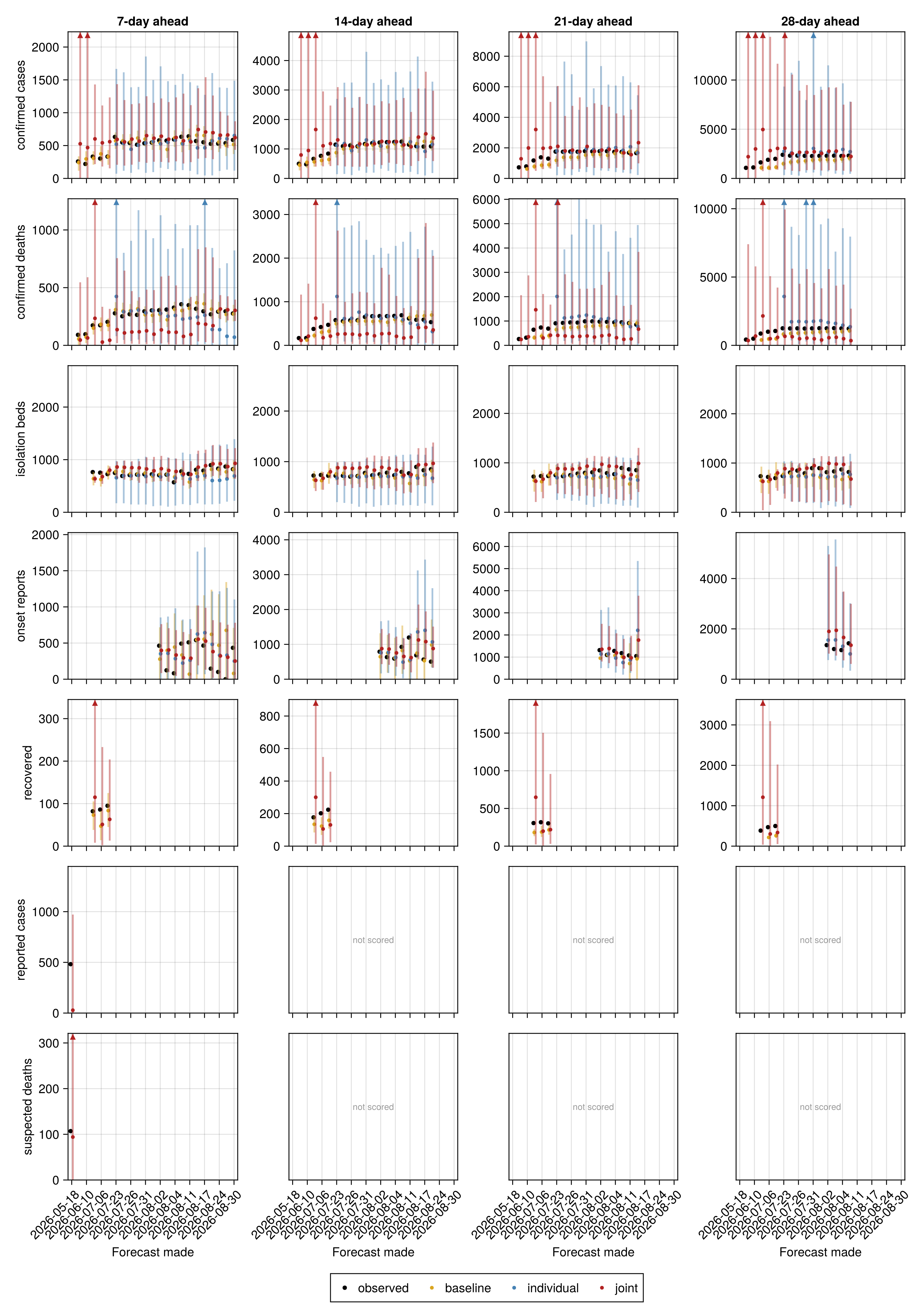
Frozen-fit forecast evaluation
The current model, frozen at earlier data cut-offs (see Forecast-versus-frozen evaluation), is scored the same way as the cross-release forecasts above, against the same persistence baseline. Only the joint model is scored here, so no individual single-stream fit appears in the tables and figures below. The May cut-offs predate the first reported bed occupancy and the first reported recoveries, so those windows are left unscored rather than scored against a series that had not started. The baseline carries a weaker data-vintage guarantee than the cross-release one, since its snapshot was taken weeks after the frozen cut-off and can hold later revisions to earlier days (see forecast scoring against a persistence baseline).
Load and summarise the frozen-fit forecast scores
frozen_scores_df = _release_data("forecast_scores_frozen.csv",
    (; release = String, made_date = Date, stream = String, horizon = Int,
        target_date = Date, fit = String, crps = Float64,
        log_crps = Float64, dispersion = Float64, overprediction = Float64,
        underprediction = Float64, coverage_50 = Float64,
        coverage_90 = Float64,
        bias = Float64, n_samples = Int,
        log_rel_to_baseline = Float64))
frozen_overlay_df = _release_data("forecast_overlay_frozen.csv",
    (; release = String, made_date = Date, stream = String, horizon = Int,
        target_date = Date, fit = String, observed = Float64,
        median = Float64, lo30 = Float64, hi30 = Float64, lo60 = Float64,
        hi60 = Float64, lo90 = Float64, hi90 = Float64))
# The frozen evaluation never carries an individual single-stream fit
# (it scores only the joint model at past cut-offs), so the individual-fit
# comparison columns are dropped rather than shown as a column of missing.
frozen_score_overview_table = drop_individual_fit_columns(
    forecast_score_overview(frozen_scores_df))
frozen_score_by_horizon_table = drop_individual_fit_columns(
    forecast_score_by_horizon(frozen_scores_df))
frozen_score_by_release_table = drop_individual_fit_columns(
    forecast_score_by_release(frozen_scores_df))

# `fit` is single-valued (`FROZEN_FIT`) by construction in every one of
# these tables, not just for the releases scored so far, so it is dropped
# from the display tables below as a degenerate column. The `..._table`
# frames above keep it and still feed the relative-skill plots, which read
# it to colour each series in the joint role.
frozen_score_overview_display = drop_degenerate_fit_column(
    frozen_score_overview_table)
frozen_score_by_horizon_display = drop_degenerate_fit_column(
    frozen_score_by_horizon_table)
# See the comment above `joint_score_by_release_table`'s assignment for why
# this setup chunk's last statement needs a trailing `;`.
frozen_score_by_release_display = drop_degenerate_fit_column(
    frozen_score_by_release_table);
The headline frozen table pools one row per stream across cut-offs and horizons, scored against the persistence baseline on both scales, with the CRPS decomposition, coverage and bias columns described above. There is no model column, since only one model is scored.
| stream | n | crps | rel_to_baseline | log_crps | log_rel_to_baseline | dispersion | overprediction | underprediction | coverage_50 | coverage_90 | bias |
|---|---|---|---|---|---|---|---|---|---|---|---|
| confirmed cases | 163 | 275.54 | 1.93 | 0.208 | 0.62 | 192.65 | 82.62 | 0.27 | 0.73 | 0.87 | 0.36 |
| confirmed deaths | 163 | 251.44 | 3.09 | 2.125 | 3.83 | 64.45 | 4.93 | 182.06 | 0.2 | 0.93 | -0.43 |
| isolation beds | 143 | 92.52 | 0.82 | 0.124 | 0.51 | 35.6 | 49.49 | 7.43 | 0.36 | 0.93 | 0.39 |
| onset reports | 29 | 173.73 | 1.04 | 0.517 | 0.78 | 72.7 | 72.33 | 28.71 | 0.41 | 0.93 | 0.15 |
| recovered | 63 | 210.77 | 2.76 | 0.474 | 2.14 | 172.58 | 34.41 | 3.78 | 0.86 | 0.89 | 0.13 |
The same relative skill against the baseline, by horizon, for the frozen cut-offs.
frozen_relative_skill_fig = plot_forecast_relative_skill(
    frozen_score_by_horizon_table);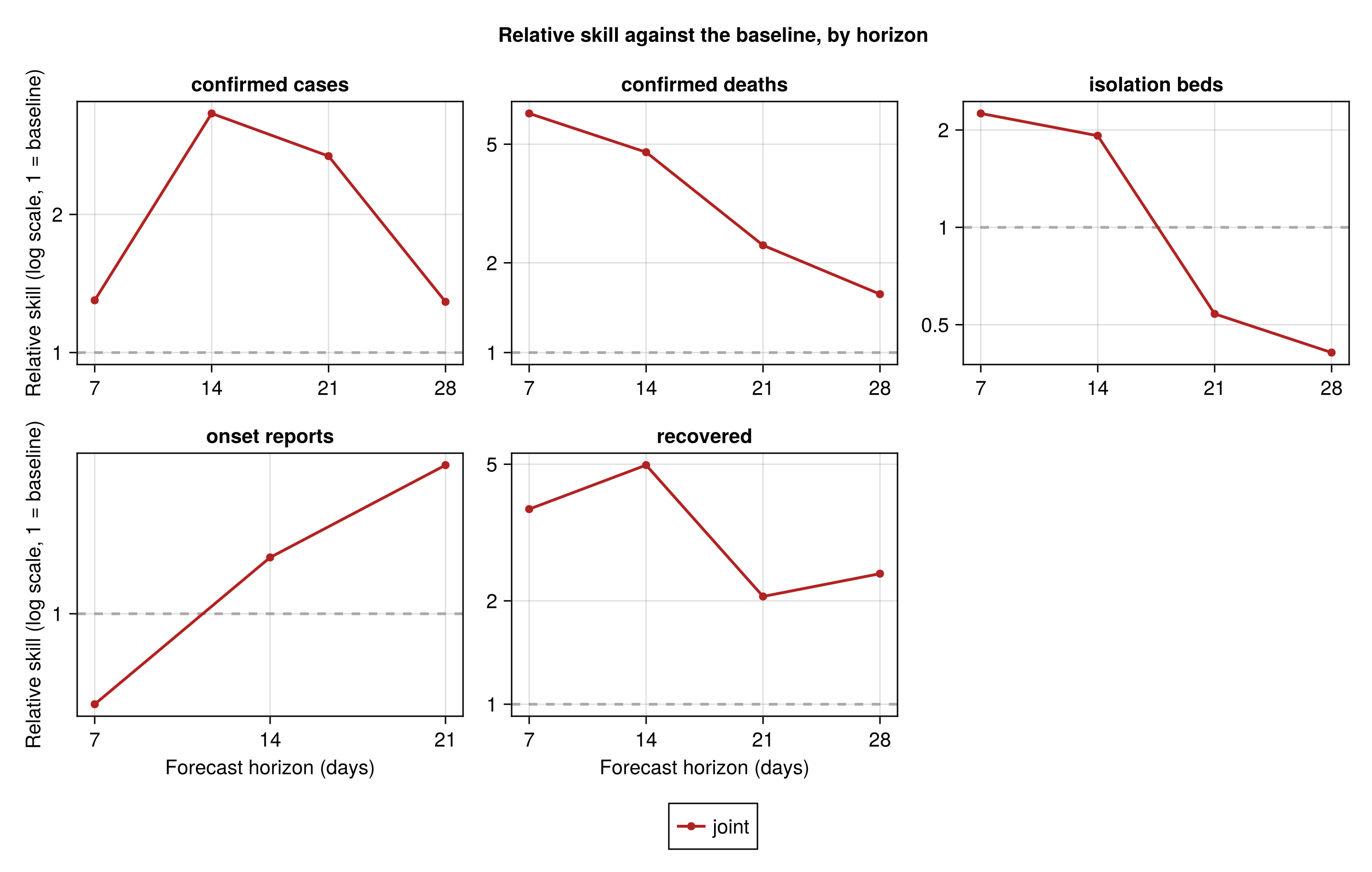
The same columns as a table, broken out by horizon, and again broken out by frozen cut-off, are behind the two dropdowns below.
Scores by horizon
| stream | horizon | n | crps | rel_to_baseline | log_crps | log_rel_to_baseline | dispersion | overprediction | underprediction | coverage_50 | coverage_90 | bias |
|---|---|---|---|---|---|---|---|---|---|---|---|---|
| confirmed cases | 7 | 80 | 110.56 | 1.3 | 0.172 | 0.34 | 70.72 | 39.29 | 0.56 | 0.7 | 0.85 | 0.35 |
| confirmed cases | 14 | 37 | 260.64 | 3.32 | 0.211 | 2.2 | 172.38 | 88.26 | 0 | 0.7 | 0.92 | 0.38 |
| confirmed cases | 21 | 34 | 510.1 | 2.68 | 0.284 | 1.52 | 343.42 | 166.68 | 0 | 0.76 | 0.82 | 0.38 |
| confirmed cases | 28 | 12 | 756.83 | 1.29 | 0.224 | 0.73 | 640.88 | 115.95 | 0 | 0.92 | 1 | 0.29 |
| confirmed deaths | 7 | 80 | 167.78 | 6.34 | 2.718 | 3.64 | 10.38 | 3.28 | 154.11 | 0.2 | 0.85 | -0.46 |
| confirmed deaths | 14 | 37 | 254.68 | 4.7 | 1.798 | 7.92 | 59 | 7.37 | 188.31 | 0.19 | 1 | -0.39 |
| confirmed deaths | 21 | 34 | 353.92 | 2.29 | 1.4 | 2.56 | 131.98 | 7.89 | 214.05 | 0.18 | 1 | -0.38 |
| confirmed deaths | 28 | 12 | 508.87 | 1.57 | 1.238 | 3.84 | 250.46 | 0 | 258.41 | 0.33 | 1 | -0.54 |
| isolation beds | 7 | 40 | 90.21 | 2.25 | 0.113 | 1.17 | 24.57 | 64.77 | 0.88 | 0.2 | 0.75 | 0.62 |
| isolation beds | 14 | 37 | 98.12 | 1.92 | 0.124 | 1.03 | 36.69 | 61.43 | 0 | 0.41 | 1 | 0.51 |
| isolation beds | 21 | 34 | 91.84 | 0.54 | 0.127 | 0.35 | 40.54 | 42.42 | 8.88 | 0.41 | 1 | 0.25 |
| isolation beds | 28 | 32 | 89.65 | 0.41 | 0.137 | 0.31 | 42.9 | 24.08 | 22.67 | 0.44 | 1 | 0.12 |
| onset reports | 7 | 14 | 124.7 | 0.69 | 0.802 | 0.73 | 51.27 | 50.55 | 22.88 | 0.43 | 0.93 | 0.09 |
| onset reports | 14 | 11 | 200.16 | 1.26 | 0.264 | 0.92 | 80.32 | 83.97 | 35.86 | 0.27 | 1 | 0.31 |
| onset reports | 21 | 4 | 272.69 | 1.84 | 0.215 | 1.35 | 126.71 | 116.51 | 29.47 | 0.75 | 0.75 | -0.05 |
| recovered | 7 | 20 | 94.64 | 3.7 | 0.499 | 2.77 | 45.5 | 46.65 | 2.49 | 0.7 | 0.8 | 0.25 |
| recovered | 14 | 17 | 178.17 | 4.97 | 0.482 | 3.56 | 106.99 | 67.38 | 3.8 | 0.82 | 0.82 | 0.18 |
| recovered | 21 | 14 | 218.83 | 2.06 | 0.439 | 1.64 | 209.3 | 3.77 | 5.76 | 1 | 1 | 0 |
| recovered | 28 | 12 | 441.1 | 2.4 | 0.461 | 1.28 | 434.45 | 3.06 | 3.59 | 1 | 1 | 0.01 |
Scores by frozen cut-off
| made_date | stream | n | crps | rel_to_baseline | log_crps | log_rel_to_baseline | dispersion | overprediction | underprediction | coverage_50 | coverage_90 | bias |
|---|---|---|---|---|---|---|---|---|---|---|---|---|
| 2026-05-23 | confirmed cases | 20 | 25.41 | 0.31 | 0.158 | 0.26 | 23.46 | 0 | 1.95 | 1 | 1 | -0.15 |
| 2026-05-27 | confirmed cases | 20 | 141.15 | 0.78 | 0.966 | 0.77 | 13.19 | 0 | 127.96 | 0 | 0.15 | -0.93 |
| 2026-06-08 | confirmed cases | 60 | 382.47 | 7.43 | 0.41 | 4.13 | 172.85 | 209.62 | 0 | 0.35 | 0.83 | 0.65 |
| 2026-07-16 | confirmed cases | 4 | 294.68 | 0.46 | 0.168 | 0.29 | 283.46 | 10.98 | 0.24 | 1 | 1 | 0.07 |
| 2026-07-18 | confirmed cases | 4 | 361.26 | 0.78 | 0.185 | 0.51 | 333.85 | 27.41 | 0 | 1 | 1 | 0.15 |
| 2026-07-19 | confirmed cases | 4 | 439.62 | 1.07 | 0.209 | 0.7 | 351.83 | 87.79 | 0 | 1 | 1 | 0.3 |
| 2026-07-20 | confirmed cases | 4 | 385.62 | 0.85 | 0.185 | 0.54 | 332.6 | 53.02 | 0 | 1 | 1 | 0.22 |
| 2026-07-24 | confirmed cases | 4 | 422.92 | 1.35 | 0.192 | 0.96 | 343.7 | 79.22 | 0 | 1 | 1 | 0.32 |
| 2026-07-25 | confirmed cases | 4 | 460.72 | 2.05 | 0.209 | 1.55 | 356.82 | 103.91 | 0 | 1 | 1 | 0.34 |
| 2026-07-26 | confirmed cases | 4 | 315.56 | 1.48 | 0.164 | 1.29 | 284.59 | 30.97 | 0 | 1 | 1 | 0.24 |
| 2026-07-27 | confirmed cases | 4 | 346.39 | 1.71 | 0.176 | 1.32 | 306.97 | 39.42 | 0 | 1 | 1 | 0.27 |
| 2026-07-28 | confirmed cases | 4 | 396.78 | 1.37 | 0.156 | 0.86 | 361.52 | 35.26 | 0 | 1 | 1 | 0.22 |
| 2026-07-31 | confirmed cases | 4 | 498.38 | 3.85 | 0.213 | 2.58 | 369.58 | 128.8 | 0 | 0.75 | 1 | 0.38 |
| 2026-08-04 | confirmed cases | 4 | 281.57 | 3.28 | 0.156 | 3.03 | 253.99 | 27.59 | 0 | 1 | 1 | 0.18 |
| 2026-08-08 | confirmed cases | 4 | 253.51 | 3.18 | 0.15 | 2.33 | 246.67 | 6.12 | 0.72 | 1 | 1 | 0.03 |
| 2026-08-10 | confirmed cases | 3 | 184.42 | 3.56 | 0.146 | 2.72 | 180.35 | 1.65 | 2.42 | 1 | 1 | -0.03 |
| 2026-08-15 | confirmed cases | 3 | 424.16 | 7.83 | 0.262 | 4.82 | 264.67 | 159.49 | 0 | 0 | 1 | 0.54 |
| 2026-08-17 | confirmed cases | 2 | 223.28 | 3.04 | 0.217 | 2.44 | 79.72 | 143.56 | 0 | 0 | 1 | 0.75 |
| 2026-08-18 | confirmed cases | 2 | 272.28 | 2.5 | 0.283 | 2.08 | 75.44 | 196.84 | 0 | 0 | 0.5 | 0.92 |
| 2026-08-23 | confirmed cases | 2 | 293.45 | 6.87 | 0.296 | 5.84 | 67.34 | 226.11 | 0 | 0 | 0.5 | 0.88 |
| 2026-08-24 | confirmed cases | 1 | 157.59 | 7.35 | 0.244 | 6.22 | 41.22 | 116.37 | 0 | 0 | 0 | 0.92 |
| 2026-08-25 | confirmed cases | 1 | 124.07 | 4.57 | 0.196 | 3.64 | 35.38 | 88.69 | 0 | 0 | 1 | 0.82 |
| 2026-08-30 | confirmed cases | 1 | 51.44 | 1.56 | 0.08 | 1.31 | 32.89 | 18.55 | 0 | 1 | 1 | 0.48 |
| 2026-05-23 | confirmed deaths | 20 | 9.42 | 0.38 | 0.431 | 0.31 | 3.42 | 0 | 6 | 0.3 | 1 | -0.56 |
| 2026-05-27 | confirmed deaths | 20 | 31.18 | 0.96 | 1.439 | 1.2 | 1.88 | 0 | 29.3 | 0 | 0.3 | -0.94 |
| 2026-06-08 | confirmed deaths | 60 | 48.52 | 0.71 | 0.219 | 0.49 | 41.95 | 5.79 | 0.78 | 0.9 | 1 | 0.03 |
| 2026-07-16 | confirmed deaths | 4 | 337 | 1.1 | 1.618 | 3.24 | 83.74 | 0 | 253.25 | 0 | 1 | -0.75 |
| 2026-07-18 | confirmed deaths | 4 | 284.84 | 1.31 | 1.516 | 4.9 | 111.23 | 0 | 173.61 | 0 | 1 | -0.66 |
| 2026-07-19 | confirmed deaths | 4 | 274.73 | 1.34 | 1.43 | 5.21 | 110.3 | 0 | 164.43 | 0 | 1 | -0.64 |
| 2026-07-20 | confirmed deaths | 4 | 312.41 | 1.44 | 1.723 | 5.75 | 107.04 | 0 | 205.38 | 0 | 1 | -0.64 |
| 2026-07-24 | confirmed deaths | 4 | 286.29 | 2.08 | 1.819 | 11.47 | 119.46 | 0 | 166.83 | 0.5 | 1 | -0.63 |
| 2026-07-25 | confirmed deaths | 4 | 303.32 | 2.52 | 1.88 | 12.76 | 135.85 | 0 | 167.47 | 0.25 | 1 | -0.58 |
| 2026-07-26 | confirmed deaths | 4 | 358.62 | 3.15 | 2.397 | 18.65 | 104.71 | 0 | 253.91 | 0 | 1 | -0.71 |
| 2026-07-27 | confirmed deaths | 4 | 363.04 | 3.18 | 2.387 | 17.17 | 146.08 | 0 | 216.96 | 0.25 | 1 | -0.58 |
| 2026-07-28 | confirmed deaths | 4 | 436.85 | 2.75 | 2.136 | 11.26 | 185.32 | 0 | 251.53 | 0 | 1 | -0.67 |
| 2026-07-31 | confirmed deaths | 4 | 351.18 | 3.11 | 2.028 | 14.84 | 172.54 | 0 | 178.64 | 0.5 | 1 | -0.57 |
| 2026-08-04 | confirmed deaths | 4 | 460.33 | 6.21 | 3.34 | 38.28 | 74.88 | 0 | 385.45 | 0 | 0.75 | -0.78 |
| 2026-08-08 | confirmed deaths | 4 | 521.22 | 7.36 | 3.723 | 34.83 | 52.58 | 0 | 468.64 | 0 | 0.75 | -0.83 |
| 2026-08-10 | confirmed deaths | 3 | 484.82 | 12.71 | 4.423 | 63.87 | 20.26 | 0 | 464.57 | 0 | 0.67 | -0.88 |
| 2026-08-15 | confirmed deaths | 3 | 272.82 | 7.21 | 2.368 | 35.52 | 150.3 | 0 | 122.52 | 0.67 | 1 | -0.47 |
| 2026-08-17 | confirmed deaths | 2 | 35.61 | 0.72 | 0.069 | 0.62 | 24.22 | 11.39 | 0 | 1 | 1 | 0.38 |
| 2026-08-18 | confirmed deaths | 2 | 51.5 | 0.77 | 0.114 | 0.72 | 23.68 | 27.83 | 0 | 0 | 1 | 0.64 |
| 2026-08-23 | confirmed deaths | 2 | 68.34 | 1.24 | 0.139 | 1.27 | 25.17 | 43.17 | 0 | 0 | 1 | 0.69 |
| 2026-08-24 | confirmed deaths | 1 | 20.13 | 1.84 | 0.063 | 1.71 | 16.61 | 3.52 | 0 | 1 | 1 | 0.29 |
| 2026-08-25 | confirmed deaths | 1 | 20.7 | 1.11 | 0.065 | 0.94 | 13.57 | 7.13 | 0 | 1 | 1 | 0.4 |
| 2026-08-30 | confirmed deaths | 1 | 21.08 | 1.62 | 0.07 | 1.41 | 13.2 | 7.88 | 0 | 1 | 1 | 0.44 |
| 2026-06-08 | isolation beds | 80 | 74.14 | 0.44 | 0.15 | 0.38 | 38.17 | 2.29 | 33.68 | 0.5 | 1 | -0.21 |
| 2026-07-16 | isolation beds | 4 | 73.22 | 2.64 | 0.096 | 2.53 | 20.01 | 53.22 | 0 | 0 | 1 | 0.6 |
| 2026-07-18 | isolation beds | 4 | 77.78 | 2.76 | 0.103 | 2.61 | 18.71 | 59.07 | 0 | 0 | 1 | 0.61 |
| 2026-07-19 | isolation beds | 4 | 100.01 | 3.47 | 0.132 | 3.31 | 22.38 | 77.63 | 0 | 0 | 1 | 0.64 |
| 2026-07-20 | isolation beds | 4 | 82.23 | 3.2 | 0.106 | 3.05 | 19.89 | 62.33 | 0 | 0.25 | 1 | 0.61 |
| 2026-07-24 | isolation beds | 4 | 76.61 | 2.77 | 0.096 | 2.59 | 10.14 | 66.47 | 0 | 0 | 1 | 0.73 |
| 2026-07-25 | isolation beds | 4 | 106.43 | 2.71 | 0.136 | 2.62 | 13.84 | 92.59 | 0 | 0 | 0.75 | 0.73 |
| 2026-07-26 | isolation beds | 4 | 94.88 | 2.44 | 0.122 | 2.32 | 22.61 | 72.27 | 0 | 0.25 | 0.75 | 0.63 |
| 2026-07-27 | isolation beds | 4 | 85.56 | 2.9 | 0.113 | 2.81 | 38.92 | 46.65 | 0 | 0.5 | 1 | 0.48 |
| 2026-07-28 | isolation beds | 4 | 153.08 | 2.77 | 0.201 | 2.48 | 41.15 | 111.94 | 0 | 0.5 | 0.75 | 0.67 |
| 2026-07-31 | isolation beds | 4 | 119.06 | 3.04 | 0.139 | 2.78 | 41.36 | 77.7 | 0 | 0.5 | 0.75 | 0.57 |
| 2026-08-04 | isolation beds | 4 | 110.51 | 1.55 | 0.153 | 1.49 | 63.26 | 47.24 | 0 | 0.75 | 0.75 | 0.42 |
| 2026-08-08 | isolation beds | 4 | 59.17 | 0.89 | 0.078 | 0.91 | 51.54 | 7.15 | 0.48 | 0.75 | 1 | 0.16 |
| 2026-08-10 | isolation beds | 3 | 46.18 | 0.87 | 0.062 | 0.87 | 45.96 | 0.02 | 0.2 | 1 | 1 | 0 |
| 2026-08-15 | isolation beds | 3 | 101.76 | 1.35 | 0.107 | 1.11 | 67.99 | 33.76 | 0 | 1 | 1 | 0.36 |
| 2026-08-17 | isolation beds | 2 | 91.77 | 3.55 | 0.1 | 3.04 | 54.51 | 37.26 | 0 | 0.5 | 1 | 0.54 |
| 2026-08-18 | isolation beds | 2 | 75.08 | 1.31 | 0.084 | 1.13 | 48.64 | 26.44 | 0 | 0.5 | 1 | 0.44 |
| 2026-08-23 | isolation beds | 2 | 128.8 | 3.94 | 0.138 | 3.54 | 47.54 | 81.27 | 0 | 0 | 1 | 0.77 |
| 2026-08-24 | isolation beds | 1 | 72.93 | 2.56 | 0.08 | 2.25 | 31.96 | 40.97 | 0 | 0 | 1 | 0.64 |
| 2026-08-25 | isolation beds | 1 | 44.53 | 0.73 | 0.054 | 0.72 | 26.99 | 0 | 17.54 | 1 | 1 | -0.49 |
| 2026-08-30 | isolation beds | 1 | 31.63 | 1.18 | 0.039 | 1.19 | 31.59 | 0 | 0.04 | 1 | 1 | -0.01 |
| 2026-07-26 | onset reports | 2 | 94.33 | 1.63 | 0.193 | 1.19 | 65.22 | 29.11 | 0 | 0.5 | 1 | 0.43 |
| 2026-07-27 | onset reports | 2 | 124.72 | 1.1 | 0.205 | 0.8 | 56.66 | 67.74 | 0.32 | 0.5 | 1 | 0.34 |
| 2026-07-28 | onset reports | 2 | 148.65 | 1.24 | 0.236 | 0.46 | 61.39 | 86.46 | 0.8 | 0.5 | 1 | 0.36 |
| 2026-07-31 | onset reports | 2 | 100.67 | 0.97 | 0.158 | 0.88 | 75.72 | 24.96 | 0 | 1 | 1 | 0.33 |
| 2026-08-04 | onset reports | 3 | 121.1 | 0.71 | 0.373 | 0.8 | 67.9 | 40.96 | 12.24 | 0.67 | 1 | 0.25 |
| 2026-08-08 | onset reports | 3 | 184.29 | 0.95 | 0.308 | 0.73 | 71.38 | 0 | 112.91 | 0.33 | 1 | -0.65 |
| 2026-08-10 | onset reports | 3 | 169.94 | 0.74 | 0.3 | 0.39 | 66.1 | 0 | 103.83 | 0.33 | 1 | -0.63 |
| 2026-08-15 | onset reports | 3 | 390.24 | 3.27 | 0.335 | 1.52 | 135.96 | 254.28 | 0 | 0.33 | 0.67 | 0.65 |
| 2026-08-17 | onset reports | 2 | 110.76 | 1.15 | 0.219 | 0.85 | 71.82 | 34.34 | 4.59 | 0.5 | 1 | 0.14 |
| 2026-08-18 | onset reports | 2 | 170.91 | 1.63 | 0.325 | 1.34 | 78.01 | 37.22 | 55.68 | 0 | 1 | -0.09 |
| 2026-08-23 | onset reports | 2 | 199.56 | 0.66 | 0.894 | 0.82 | 66.89 | 132.68 | 0 | 0 | 1 | 0.71 |
| 2026-08-24 | onset reports | 1 | 125.58 | 0.5 | 0.699 | 0.69 | 62.25 | 63.33 | 0 | 0 | 1 | 0.59 |
| 2026-08-25 | onset reports | 1 | 358.63 | 0.72 | 5.707 | 1.02 | 35.28 | 323.35 | 0 | 0 | 0 | 0.99 |
| 2026-08-30 | onset reports | 1 | 58.19 | 0.31 | 0.166 | 0.11 | 35.24 | 0 | 22.95 | 1 | 1 | -0.48 |
| 2026-07-16 | recovered | 4 | 139.34 | 1.1 | 0.469 | 1.09 | 135.5 | 0 | 3.84 | 1 | 1 | -0.1 |
| 2026-07-18 | recovered | 4 | 149.61 | 2.29 | 0.455 | 2.24 | 146.94 | 2.67 | 0 | 1 | 1 | 0.1 |
| 2026-07-19 | recovered | 4 | 181.47 | 2.24 | 0.482 | 2.11 | 179.35 | 2.12 | 0 | 1 | 1 | 0.07 |
| 2026-07-20 | recovered | 4 | 171.81 | 2.13 | 0.417 | 1.93 | 169.63 | 2.18 | 0 | 1 | 1 | 0.06 |
| 2026-07-24 | recovered | 4 | 179.37 | 2.26 | 0.409 | 1.93 | 175.36 | 4.01 | 0 | 1 | 1 | 0.13 |
| 2026-07-25 | recovered | 4 | 177.7 | 2.04 | 0.379 | 1.64 | 173.52 | 4.18 | 0 | 1 | 1 | 0.12 |
| 2026-07-26 | recovered | 4 | 139.99 | 1.51 | 0.381 | 1.57 | 138.99 | 0 | 1 | 1 | 1 | -0.05 |
| 2026-07-27 | recovered | 4 | 219.87 | 2.19 | 0.483 | 1.81 | 218.38 | 0 | 1.49 | 1 | 1 | -0.06 |
| 2026-07-28 | recovered | 4 | 544.07 | 3.75 | 0.369 | 0.83 | 543.25 | 0.5 | 0.33 | 1 | 1 | 0.02 |
| 2026-07-31 | recovered | 4 | 249.16 | 2.39 | 0.402 | 1.48 | 242.91 | 6.25 | 0 | 1 | 1 | 0.12 |
| 2026-08-04 | recovered | 4 | 157.98 | 2.31 | 0.457 | 2.71 | 146.41 | 0 | 11.57 | 1 | 1 | -0.19 |
| 2026-08-08 | recovered | 4 | 125.59 | 1.62 | 0.417 | 2.13 | 109.72 | 0 | 15.87 | 1 | 1 | -0.23 |
| 2026-08-10 | recovered | 3 | 119.75 | 1.97 | 0.524 | 2.58 | 85.84 | 0 | 33.9 | 1 | 1 | -0.32 |
| 2026-08-15 | recovered | 3 | 241.64 | 13.11 | 0.412 | 6.36 | 212.86 | 28.78 | 0 | 1 | 1 | 0.28 |
| 2026-08-17 | recovered | 2 | 309.21 | 12.68 | 0.773 | 6.65 | 57.82 | 251.39 | 0 | 0 | 0 | 0.92 |
| 2026-08-18 | recovered | 2 | 342.31 | 15.63 | 0.823 | 7.84 | 52.64 | 289.67 | 0 | 0 | 0 | 0.94 |
| 2026-08-23 | recovered | 2 | 303.49 | 25.25 | 0.698 | 12.8 | 59.73 | 243.76 | 0 | 0 | 0.5 | 0.9 |
| 2026-08-24 | recovered | 1 | 187.31 | 18.08 | 0.698 | 10.51 | 40.92 | 146.39 | 0 | 0 | 0 | 0.92 |
| 2026-08-25 | recovered | 1 | 182.96 | 16.99 | 0.67 | 9.83 | 39.71 | 143.25 | 0 | 0 | 0 | 0.93 |
| 2026-08-30 | recovered | 1 | 170.25 | 17.02 | 0.609 | 10.26 | 35.53 | 134.72 | 0 | 0 | 1 | 0.86 |
The frozen forecasts made at each cut-off against the value observed since, one panel per stream and horizon, the observed value in black. Each panel carries the frozen forecast and the persistence baseline, coloured as in the cross-release overlay above, and the x-axis is the cut-off each forecast was made from. The same per-panel axis crop and overflow marker applies here.
Frozen-fit forecasts-versus-now overlay
frozen_overlay_fig = plot_forecast_overlay(frozen_overlay_df);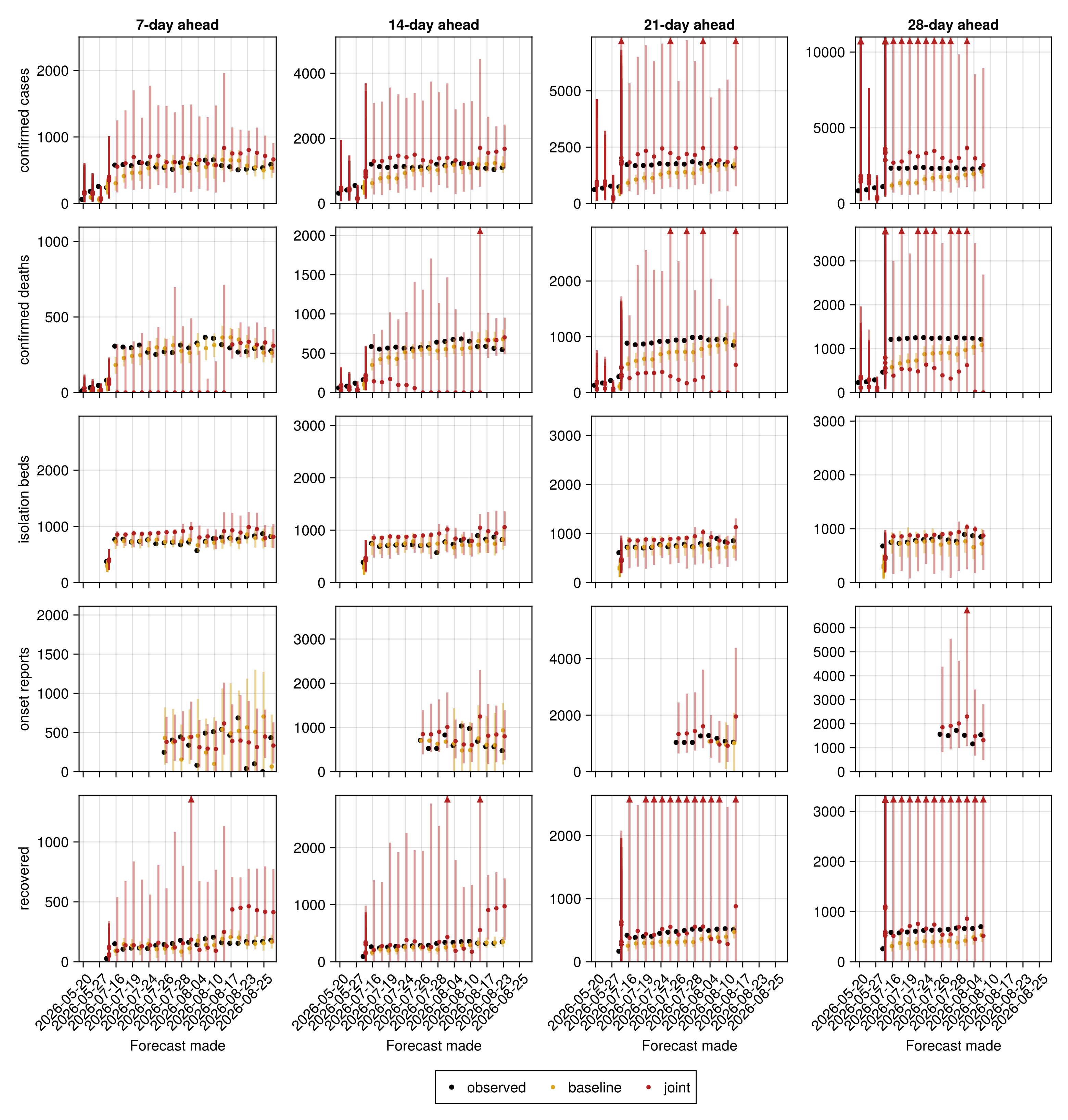
The frozen re-fits below freeze the renewal data to an earlier cut-off and re-fit, so that a change driven by newer data can be distinguished from one driven by a change of method. Each uses the full headline settings: 1000 draws across two chains.
Freeze the renewal data to a cut-off and re-fit
# Frozen re-fits and released_df are prepared in the setup block above.Individual fits against the baseline
This section carries the same cross-release forecast scoring as Forecast scoring across releases above, for each stream's own individual fit rather than the joint, against the same persistence baseline. Recovered has no individual fit, so it does not appear here. These are the individual-fit rows of the same scored forecasts, not a separate computation. Only the newest few releases carry an individual-stream forecast, so these tables cover those releases alone rather than the outbreak's history.
Individual-fit rows of the cross-release scores
# The relative skill against a stream's individual fit is only ever
# computed on the joint model's row, so on these rows it is missing by
# construction and the column is dropped rather than shown empty.
individual_score_overview_table = drop_individual_fit_columns(
    select_fit_role(forecast_score_overview_table, "individual"))
individual_score_by_horizon_table = drop_individual_fit_columns(
    select_fit_role(forecast_score_by_horizon_table, "individual"))
# See the comment above `joint_score_by_release_table`'s assignment for why
# this setup chunk's last statement needs a trailing `;`.
individual_score_by_release_table = drop_individual_fit_columns(
select_fit_role(forecast_score_by_release_table, "individual"));| stream | fit | n | crps | rel_to_baseline | log_crps | log_rel_to_baseline | dispersion | overprediction | underprediction | coverage_50 | coverage_90 | bias |
|---|---|---|---|---|---|---|---|---|---|---|---|---|
| confirmed cases | confirmed | 53 | 285.74 | 1.93 | 0.193 | 1.88 | 275 | 8.71 | 2.04 | 1 | 1 | 0.02 |
| confirmed deaths | confirmed_deaths | 53 | 264.86 | 2.82 | 0.324 | 2.59 | 223.58 | 35.36 | 5.92 | 0.91 | 1 | 0.03 |
| isolation beds | treatment | 53 | 86.49 | 1.61 | 0.14 | 1.93 | 73.26 | 0.11 | 13.12 | 0.94 | 1 | -0.21 |
| onset reports | onsets | 25 | 229.42 | 1.22 | 0.534 | 0.78 | 109.8 | 77.78 | 41.84 | 0.4 | 0.96 | 0.09 |
The same relative skill against the baseline, by horizon, one panel per stream (dataset), for each stream's own individual fit.
individual_relative_skill_fig = plot_forecast_relative_skill(
    individual_score_by_horizon_table;
    empty_message = "Empty: no release old enough for its targets to " *
                    "have been observed carries an individual-stream " *
                    "forecast. Not a missing forecast.");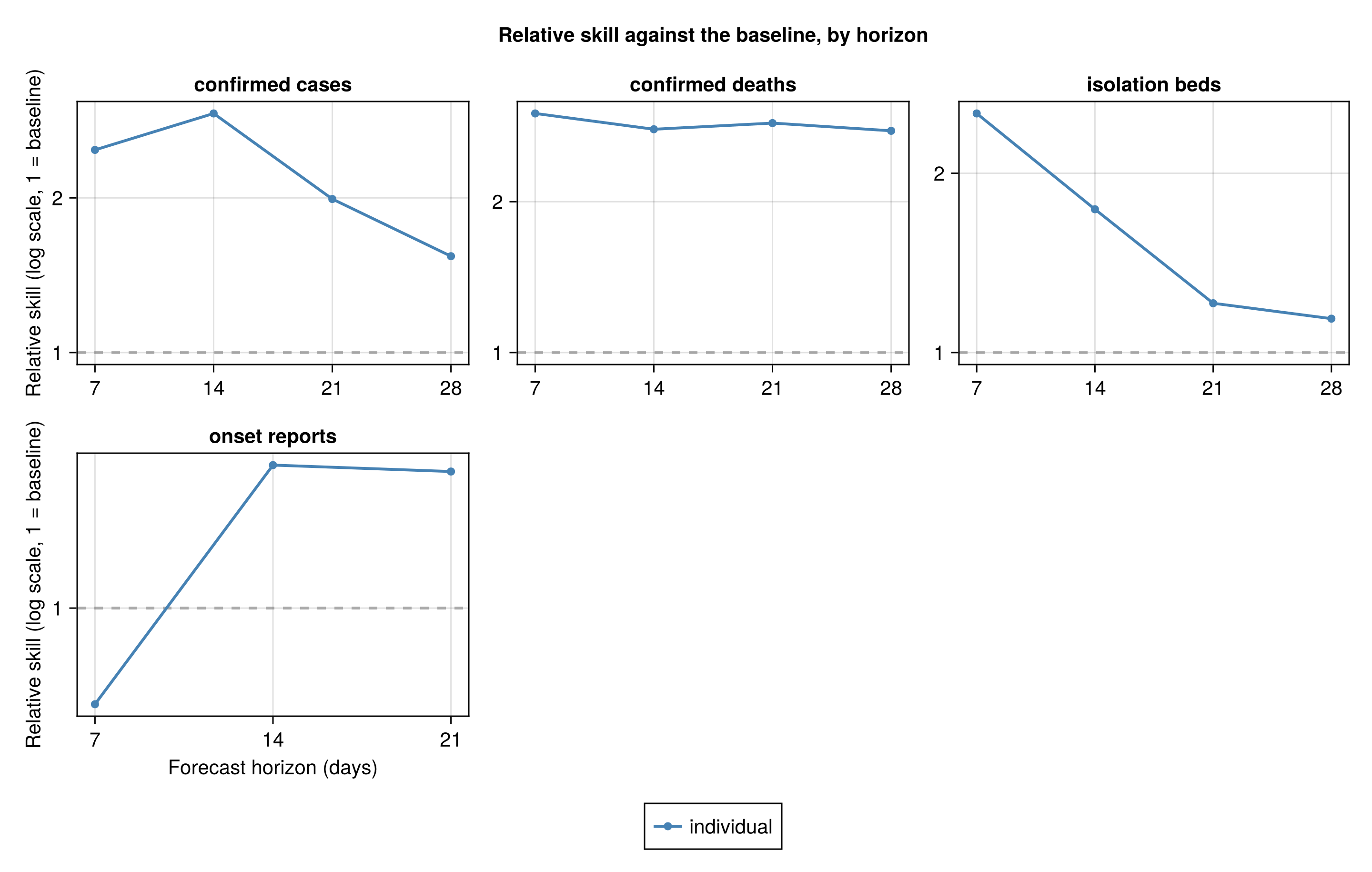
The same columns as a table, broken out by horizon, and again broken out by release, are behind the two dropdowns below.
Scores by horizon
| stream | horizon | fit | n | crps | rel_to_baseline | log_crps | log_rel_to_baseline | dispersion | overprediction | underprediction | coverage_50 | coverage_90 | bias |
|---|---|---|---|---|---|---|---|---|---|---|---|---|---|
| confirmed cases | 7 | confirmed | 17 | 97.18 | 2.48 | 0.181 | 2.6 | 92.22 | 1.37 | 3.59 | 1 | 1 | -0.04 |
| confirmed cases | 14 | confirmed | 14 | 213.22 | 2.92 | 0.189 | 2.87 | 208.53 | 1.41 | 3.28 | 1 | 1 | -0.02 |
| confirmed cases | 21 | confirmed | 12 | 369.43 | 1.99 | 0.196 | 1.67 | 361.41 | 7.93 | 0.09 | 1 | 1 | 0.07 |
| confirmed cases | 28 | confirmed | 10 | 607.41 | 1.54 | 0.218 | 1.13 | 575.08 | 32.33 | 0 | 1 | 1 | 0.14 |
| confirmed deaths | 7 | confirmed_deaths | 17 | 77.34 | 3 | 0.359 | 4.11 | 60.79 | 1.92 | 14.63 | 0.88 | 1 | -0.16 |
| confirmed deaths | 14 | confirmed_deaths | 14 | 169.77 | 2.79 | 0.287 | 2.85 | 154.36 | 11.77 | 3.64 | 0.93 | 1 | 0.01 |
| confirmed deaths | 21 | confirmed_deaths | 12 | 332.83 | 2.87 | 0.305 | 2.25 | 293.89 | 37.78 | 1.17 | 0.92 | 1 | 0.11 |
| confirmed deaths | 28 | confirmed_deaths | 10 | 635.2 | 2.77 | 0.34 | 1.61 | 512.86 | 122.34 | 0 | 0.9 | 1 | 0.27 |
| isolation beds | 7 | treatment | 17 | 93.36 | 2.52 | 0.155 | 3.03 | 80.89 | 0.27 | 12.19 | 1 | 1 | -0.16 |
| isolation beds | 14 | treatment | 14 | 84.07 | 1.74 | 0.138 | 2.09 | 76.37 | 0.08 | 7.62 | 1 | 1 | -0.15 |
| isolation beds | 21 | treatment | 12 | 83.5 | 1.21 | 0.133 | 1.43 | 68.08 | 0 | 15.42 | 0.92 | 1 | -0.25 |
| isolation beds | 28 | treatment | 10 | 81.79 | 1.14 | 0.125 | 1.33 | 62.13 | 0 | 19.66 | 0.8 | 1 | -0.37 |
| onset reports | 7 | onsets | 11 | 139.13 | 0.7 | 0.816 | 0.67 | 79.32 | 40.36 | 19.45 | 0.36 | 1 | 0.16 |
| onset reports | 14 | onsets | 8 | 301.4 | 1.7 | 0.368 | 1.26 | 116.28 | 119.33 | 65.78 | 0.38 | 0.88 | 0.15 |
| onset reports | 21 | onsets | 6 | 298.97 | 1.66 | 0.236 | 1.15 | 157.03 | 90.98 | 50.96 | 0.5 | 1 | -0.11 |
Scores by release
| made_date | stream | fit | n | crps | rel_to_baseline | log_crps | log_rel_to_baseline | dispersion | overprediction | underprediction | coverage_50 | coverage_90 | bias |
|---|---|---|---|---|---|---|---|---|---|---|---|---|---|
| 2026-07-23 | confirmed cases | confirmed | 4 | 327.81 | 0.84 | 0.206 | 0.81 | 319.43 | 4.84 | 3.55 | 1 | 1 | -0.03 |
| 2026-07-25 | confirmed cases | confirmed | 4 | 346.24 | 1.53 | 0.213 | 1.57 | 343.88 | 2.3 | 0.06 | 1 | 1 | 0.02 |
| 2026-07-26 | confirmed cases | confirmed | 4 | 299.07 | 1.36 | 0.211 | 1.59 | 291.39 | 0.16 | 7.51 | 1 | 1 | -0.12 |
| 2026-07-27 | confirmed cases | confirmed | 4 | 267.62 | 1.32 | 0.171 | 1.3 | 262.03 | 5.38 | 0.21 | 1 | 1 | 0.04 |
| 2026-07-31 | confirmed cases | confirmed | 4 | 402.87 | 2.88 | 0.219 | 2.49 | 383.82 | 19.05 | 0 | 1 | 1 | 0.09 |
| 2026-08-01 | confirmed cases | confirmed | 4 | 336.31 | 2.87 | 0.209 | 3 | 322.98 | 13.33 | 0 | 1 | 1 | 0.08 |
| 2026-08-02 | confirmed cases | confirmed | 4 | 296.98 | 2.26 | 0.171 | 2.05 | 286.15 | 6.72 | 4.11 | 1 | 1 | -0.03 |
| 2026-08-03 | confirmed cases | confirmed | 4 | 291.8 | 1.52 | 0.175 | 1.2 | 281.42 | 10.08 | 0.3 | 1 | 1 | 0.05 |
| 2026-08-04 | confirmed cases | confirmed | 4 | 350.84 | 3.84 | 0.191 | 3.45 | 323.41 | 27.4 | 0.04 | 1 | 1 | 0.11 |
| 2026-08-07 | confirmed cases | confirmed | 4 | 308.4 | 3.45 | 0.192 | 2.75 | 294.77 | 9.51 | 4.12 | 1 | 1 | -0.01 |
| 2026-08-11 | confirmed cases | confirmed | 3 | 235.24 | 5.57 | 0.183 | 4.71 | 220.42 | 13.71 | 1.11 | 1 | 1 | 0.06 |
| 2026-08-15 | confirmed cases | confirmed | 3 | 216.85 | 4.13 | 0.202 | 3.84 | 213.73 | 0 | 3.12 | 1 | 1 | -0.06 |
| 2026-08-17 | confirmed cases | confirmed | 2 | 144.46 | 1.65 | 0.209 | 2.06 | 136.61 | 0 | 7.84 | 1 | 1 | -0.15 |
| 2026-08-22 | confirmed cases | confirmed | 2 | 159.72 | 2.91 | 0.192 | 3.14 | 157.83 | 1.89 | 0 | 1 | 1 | 0.07 |
| 2026-08-24 | confirmed cases | confirmed | 1 | 88.92 | 3.75 | 0.156 | 3.58 | 82.49 | 6.43 | 0 | 1 | 1 | 0.14 |
| 2026-08-25 | confirmed cases | confirmed | 1 | 90.86 | 3.54 | 0.158 | 3.1 | 84.13 | 6.73 | 0 | 1 | 1 | 0.2 |
| 2026-08-30 | confirmed cases | confirmed | 1 | 88.04 | 2.02 | 0.138 | 1.71 | 79.79 | 8.25 | 0 | 1 | 1 | 0.21 |
| 2026-07-23 | confirmed deaths | confirmed_deaths | 4 | 701.54 | 4.31 | 0.448 | 2.27 | 383.29 | 318.25 | 0 | 0.25 | 1 | 0.56 |
| 2026-07-25 | confirmed deaths | confirmed_deaths | 4 | 237.78 | 1.95 | 0.234 | 1.58 | 214.28 | 23.5 | 0 | 1 | 1 | 0.18 |
| 2026-07-26 | confirmed deaths | confirmed_deaths | 4 | 256.46 | 2.2 | 0.255 | 1.91 | 231.65 | 24.81 | 0 | 1 | 1 | 0.13 |
| 2026-07-27 | confirmed deaths | confirmed_deaths | 4 | 310.27 | 2.84 | 0.252 | 1.88 | 280.84 | 29.43 | 0 | 1 | 1 | 0.21 |
| 2026-07-31 | confirmed deaths | confirmed_deaths | 4 | 312.36 | 2.63 | 0.289 | 2.05 | 292.21 | 20.08 | 0.07 | 1 | 1 | 0.08 |
| 2026-08-01 | confirmed deaths | confirmed_deaths | 4 | 280.92 | 2.41 | 0.253 | 1.73 | 261.46 | 19.46 | 0 | 1 | 1 | 0.1 |
| 2026-08-02 | confirmed deaths | confirmed_deaths | 4 | 256.05 | 2.83 | 0.276 | 2.38 | 238.23 | 16.88 | 0.94 | 1 | 1 | 0.03 |
| 2026-08-03 | confirmed deaths | confirmed_deaths | 4 | 224.5 | 1.64 | 0.245 | 1.23 | 212.2 | 10.83 | 1.46 | 1 | 1 | 0.02 |
| 2026-08-04 | confirmed deaths | confirmed_deaths | 4 | 248.77 | 3.27 | 0.283 | 3.16 | 242.12 | 4.29 | 2.35 | 1 | 1 | -0.02 |
| 2026-08-07 | confirmed deaths | confirmed_deaths | 4 | 231.5 | 3.06 | 0.325 | 2.97 | 223.68 | 1.02 | 6.79 | 1 | 1 | -0.11 |
| 2026-08-11 | confirmed deaths | confirmed_deaths | 3 | 166.04 | 7.83 | 0.329 | 8.55 | 153.95 | 0 | 12.09 | 1 | 1 | -0.2 |
| 2026-08-15 | confirmed deaths | confirmed_deaths | 3 | 169.78 | 4.08 | 0.331 | 4.53 | 163.26 | 0 | 6.52 | 1 | 1 | -0.14 |
| 2026-08-17 | confirmed deaths | confirmed_deaths | 2 | 108.79 | 2.18 | 0.271 | 2.4 | 106.19 | 0 | 2.6 | 1 | 1 | -0.12 |
| 2026-08-22 | confirmed deaths | confirmed_deaths | 2 | 130.72 | 1.79 | 0.483 | 3.36 | 111.26 | 0 | 19.46 | 1 | 1 | -0.22 |
| 2026-08-24 | confirmed deaths | confirmed_deaths | 1 | 94.67 | 8.56 | 0.566 | 15.27 | 46.89 | 0 | 47.78 | 1 | 1 | -0.49 |
| 2026-08-25 | confirmed deaths | confirmed_deaths | 1 | 106.13 | 6.56 | 0.799 | 13.52 | 51.28 | 0 | 54.85 | 0 | 1 | -0.55 |
| 2026-08-30 | confirmed deaths | confirmed_deaths | 1 | 109.76 | 10.96 | 0.904 | 24.65 | 45.13 | 0 | 64.63 | 0 | 1 | -0.55 |
| 2026-07-23 | isolation beds | treatment | 4 | 55.73 | 1.89 | 0.089 | 2.3 | 47.79 | 0 | 7.94 | 1 | 1 | -0.21 |
| 2026-07-25 | isolation beds | treatment | 4 | 51.68 | 1.4 | 0.082 | 1.68 | 47.14 | 0.01 | 4.52 | 1 | 1 | -0.14 |
| 2026-07-26 | isolation beds | treatment | 4 | 61.67 | 1.64 | 0.1 | 1.98 | 54.82 | 0.23 | 6.63 | 1 | 1 | -0.12 |
| 2026-07-27 | isolation beds | treatment | 4 | 59.47 | 2.05 | 0.098 | 2.47 | 54.67 | 0 | 4.8 | 1 | 1 | -0.18 |
| 2026-07-31 | isolation beds | treatment | 4 | 82.76 | 1.95 | 0.132 | 2.43 | 68.17 | 0 | 14.6 | 0.75 | 1 | -0.28 |
| 2026-08-01 | isolation beds | treatment | 4 | 88.62 | 1.38 | 0.153 | 1.78 | 73.94 | 0 | 14.67 | 0.75 | 1 | -0.25 |
| 2026-08-02 | isolation beds | treatment | 4 | 84.37 | 1.65 | 0.141 | 2.03 | 69.7 | 0 | 14.67 | 0.75 | 1 | -0.28 |
| 2026-08-03 | isolation beds | treatment | 4 | 79.93 | 1.88 | 0.134 | 2.32 | 71.91 | 0 | 8.01 | 1 | 1 | -0.21 |
| 2026-08-04 | isolation beds | treatment | 4 | 87.06 | 1.23 | 0.141 | 1.39 | 82.73 | 1.22 | 3.11 | 1 | 1 | -0.03 |
| 2026-08-07 | isolation beds | treatment | 4 | 104.98 | 1.81 | 0.171 | 2.26 | 85.76 | 0 | 19.21 | 1 | 1 | -0.29 |
| 2026-08-11 | isolation beds | treatment | 3 | 103.68 | 0.63 | 0.173 | 0.72 | 89.95 | 0 | 13.73 | 1 | 1 | -0.22 |
| 2026-08-15 | isolation beds | treatment | 3 | 123.88 | 1.62 | 0.198 | 2.03 | 95.9 | 0 | 27.98 | 1 | 1 | -0.31 |
| 2026-08-17 | isolation beds | treatment | 2 | 98.59 | 2.09 | 0.158 | 2.54 | 90.9 | 0 | 7.69 | 1 | 1 | -0.18 |
| 2026-08-22 | isolation beds | treatment | 2 | 144.28 | 3.57 | 0.22 | 4.54 | 106.64 | 0 | 37.65 | 1 | 1 | -0.3 |
| 2026-08-24 | isolation beds | treatment | 1 | 134.63 | 5.57 | 0.216 | 7.18 | 100.67 | 0 | 33.96 | 1 | 1 | -0.36 |
| 2026-08-25 | isolation beds | treatment | 1 | 137.86 | 2.32 | 0.205 | 2.8 | 103.65 | 0 | 34.21 | 1 | 1 | -0.26 |
| 2026-08-30 | isolation beds | treatment | 1 | 117.98 | 4.92 | 0.172 | 5.81 | 99.19 | 0 | 18.79 | 1 | 1 | -0.25 |
| 2026-08-02 | onset reports | onsets | 3 | 111.07 | 0.59 | 0.178 | 0.55 | 96.84 | 0 | 14.23 | 1 | 1 | -0.2 |
| 2026-08-03 | onset reports | onsets | 3 | 135.35 | 1.5 | 0.312 | 1.08 | 100.32 | 35.03 | 0 | 0.67 | 1 | 0.36 |
| 2026-08-04 | onset reports | onsets | 3 | 138.85 | 0.79 | 0.369 | 0.73 | 88.34 | 16.71 | 33.8 | 0.33 | 1 | 0.01 |
| 2026-08-07 | onset reports | onsets | 3 | 221.05 | 1.88 | 0.467 | 2.37 | 82.32 | 0 | 138.73 | 0 | 1 | -0.63 |
| 2026-08-11 | onset reports | onsets | 3 | 237.9 | 0.77 | 0.436 | 0.48 | 85.91 | 0 | 151.99 | 0.33 | 1 | -0.59 |
| 2026-08-15 | onset reports | onsets | 3 | 486.37 | 4.02 | 0.388 | 1.82 | 205.04 | 281.33 | 0 | 0.33 | 1 | 0.62 |
| 2026-08-17 | onset reports | onsets | 2 | 374.54 | 3.81 | 0.44 | 1.82 | 153.61 | 220.93 | 0 | 0.5 | 0.5 | 0.63 |
| 2026-08-22 | onset reports | onsets | 2 | 271.95 | 0.91 | 0.583 | 0.85 | 104.12 | 167.83 | 0 | 0 | 1 | 0.69 |
| 2026-08-24 | onset reports | onsets | 1 | 143.07 | 0.62 | 0.764 | 0.77 | 82.09 | 60.98 | 0 | 0 | 1 | 0.52 |
| 2026-08-25 | onset reports | onsets | 1 | 195.35 | 0.42 | 3.405 | 0.64 | 88.57 | 106.78 | 0 | 0 | 1 | 0.79 |
| 2026-08-30 | onset reports | onsets | 1 | 112.25 | 0.6 | 0.676 | 0.44 | 82.46 | 0 | 29.79 | 1 | 1 | -0.37 |
Outbreak size estimated by each data stream
Each data stream constrains the latent outbreak size differently. The table below puts the posteriors over the infection count side by side, the single-stream fits and the joint, to show what each stream implies alone and what the joint adds.
Per-stream infection-count table
streams_C_table = streams_table(
    "exports" => posterior_C_exports,
    "deaths (DRC)" => posterior_C_deaths,
    "cases (DRC)" => posterior_C_cases,
    "confirmed (DRC)" => posterior_C_confirmed,
    "isolation (DRC)" => posterior_C_treatment,
    "onsets (DRC)" => posterior_C_onsets,
"joint" => posterior_C_joint);| Stream | Lower 90% | Lower 60% | Lower 30% | Upper 30% | Upper 60% | Upper 90% |
|---|---|---|---|---|---|---|
| exports | 3932 | 15558 | 47451 | 347159 | 1157555 | 39941175 |
| deaths (DRC) | 26984 | 44995 | 62414 | 106314 | 149314 | 331276 |
| cases (DRC) | 30136 | 37079 | 41983 | 55230 | 67232 | 114167 |
| confirmed (DRC) | 50324 | 60772 | 69849 | 95426 | 117564 | 205410 |
| isolation (DRC) | 11614 | 13427 | 14991 | 19032 | 23476 | 42249 |
| onsets (DRC) | 19042 | 27811 | 35940 | 61011 | 83812 | 149746 |
| joint | 9749 | 11206 | 12399 | 14531 | 16111 | 19236 |
The first figure shows each single-stream fit's cumulative-infection trajectory projected to the cut-off, with a dotted rule in each stream's colour marking where its data stops and the ribbon beyond it becomes a forward projection.
Per-stream projected-trajectory plot
# Per-draw cumulative-infection trajectory carried by each single-stream
# fit out to the cut-off on day `n`, so streams whose data ends earlier are
# still projected to today.
function _cuminf(chn)
    mat = chn[:cumulative_infections]
    return [collect(v) for v in vec(collect(mat))]
end
# Grid day a stream's data last reports, used for the dotted rule. The
# suspected case and death histories freeze at 26 May; exports and confirmed
# run to the cut-off.
_last_day(days) = isempty(days) ? nothing : maximum(days)

stream_traj_fig = plot_stream_trajectories(
    [
        (; label = "exports", trajs = _cuminf(chn_exports),
            last_day = _last_day(vcat(obs.export_case_days,
                obs.export_death_days)), colour = :seagreen),
        (; label = "deaths (DRC)", trajs = _cuminf(chn_deaths),
            last_day = _last_day(obs.deaths_history.days),
            colour = :firebrick),
        (; label = "cases (DRC)", trajs = _cuminf(chn_cases),
            last_day = _last_day(obs.reported_history.days),
            colour = :steelblue),
        (; label = "confirmed (DRC)", trajs = _cuminf(chn_confirmed),
            last_day = _last_day(obs.confirmed_history.days),
            colour = :goldenrod),
        (; label = "isolation (DRC)", trajs = _cuminf(chn_treatment),
            last_day = _last_day(obs.isolation_history.days),
            colour = :darkorange),
        (; label = "onsets (DRC)", trajs = _cuminf(chn_onsets),
            last_day = _last_day(obs.onset_curve_history.report_days),
            colour = :mediumpurple)];
    n = obs.n, seeding = obs.seeding);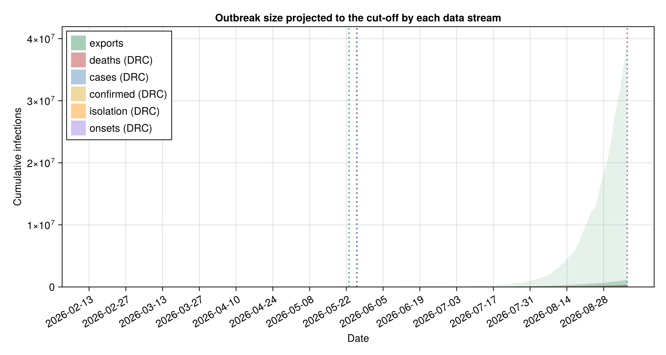
The second figure is the posterior density of each fit's cumulative infection count at the cut-off. The x-axis is scaled to a multiple of the joint-fit 90% upper bound so the bulk of the streams stays visible rather than being flattened by the wide, ill-defined confirmed-only tail.
Cut-off infection-count density plot
# Scale the x-axis to twice the joint-fit 90% upper bound, so the joint and
# the streams that track it read clearly while the confirmed-only tail runs
# off the axis rather than dominating it.
density_xmax = 2.0 * quantile(posterior_C_joint, 0.95)

cumulative_density_fig = plot_cumulative_cases(
    "exports" => posterior_C_exports,
    "deaths (DRC)" => posterior_C_deaths,
    "cases (DRC)" => posterior_C_cases,
    "confirmed (DRC)" => posterior_C_confirmed,
    "isolation (DRC)" => posterior_C_treatment,
    "onsets (DRC)" => posterior_C_onsets,
    "joint" => posterior_C_joint;
    scenarios = [], xmax = density_xmax);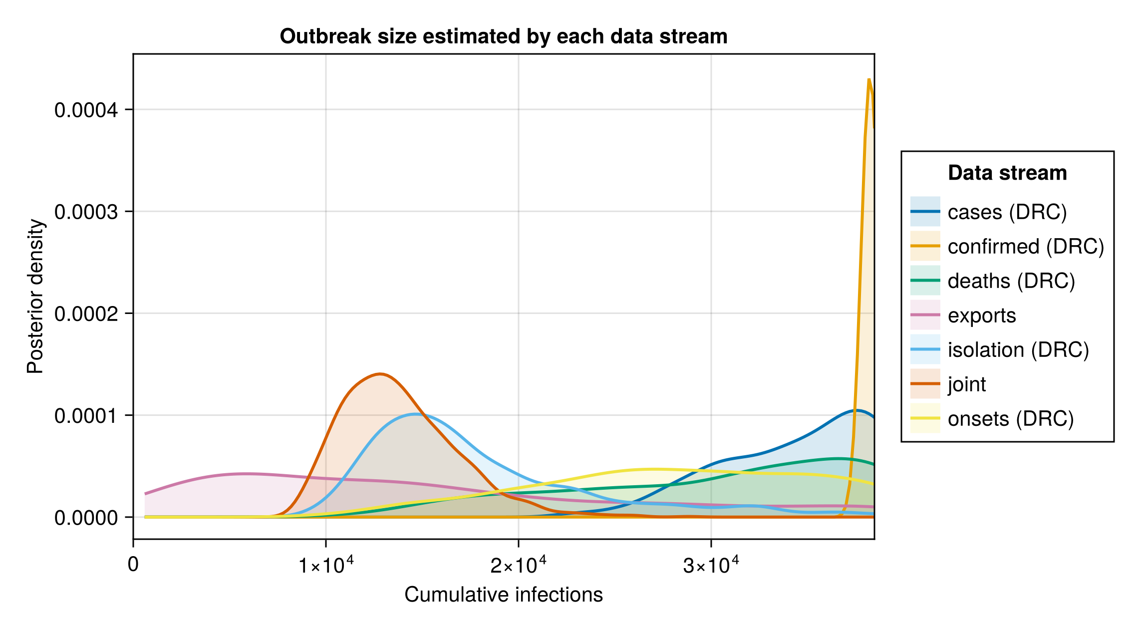
Estimate evolution across releases
How the outbreak-size estimate has moved as situation reports accrued, three series on one calendar axis. The estimate published at each release is in blue, drawn as a median with nested 30/60/90% interval bars because each release is its own fit rather than one continuous model. The current model frozen at earlier cut-offs is in red, reusing fits already made for the McCabe and Chamla comparisons and the forecast validation. The current model on current data is the green band, drawn day by day so the latest estimate reads against the earlier points. Dotted vertical rules mark the release dates. The published series switches from a closed-form integral model to a renewal model on 7 June, so a step there can reflect the change of method rather than of data.
Released estimates and the current-model frozen re-fits
# Released median and 30/60/90% intervals per release, from
# `data/released_estimates.csv`. Each tuple is
# `(date, median, lo30, hi30, lo60, hi60, lo90, hi90)`.
release_evolution = [(string(r.date), r.median, r.lo30, r.hi30, r.lo60, r.hi60,
                         r.lo90, r.hi90) for r in eachrow(released_df)]

# The current model frozen at earlier cut-offs, each its own discrete
# estimate: the matched-McCabe cut-offs (20, 23, 27 May) already computed
# for the matched-in-time comparison below, the 8 June Chamla
# confirmed-case anchor computed for the Chamla comparison, and the
# one-week-back validation fit (`frozen_lastweek`, at `validation_cutoff`)
# already computed for the forecast validation above. All are reused here so
# the current-model estimate at those earlier cut-offs reads against the
# released overlay, including a recent point one week before the cut-off.
# No extra fits are run. Each tuple carries the median and 30/60/90%
# credible bounds from the frozen draws; `round_fn` rounds to a whole count
# for outbreak size, and is passed through unrounded for a continuous
# quantity such as R0.
function _ci369(xs; round_fn = x -> round(Int, x))
    q(p) = round_fn(quantile(xs, p))
    (q(0.5), q(0.35), q(0.65), q(0.20), q(0.80), q(0.05), q(0.95))
end
frozen_by_cutoff[validation_cutoff] = frozen_lastweek
# The cut-offs every frozen fit above was made at, shared by the
# outbreak-size and R0 by-release overlays below.
_frozen_matched_cutoffs = sort(union(frozen_cutoffs,
    [validation_cutoff, default_chamla_cutoff()]))
frozen_matched = [(c, _ci369(frozen_C(c))...) for c in _frozen_matched_cutoffs]

# The current-data, current-model estimate as the cumulative-infection
# trajectory over the day grid (one calendar date per grid day, day 1 is
# the seeding date), summarised by per-day 30/60/90% credible bounds. This
# is the same latent quantity the cumulative-trajectory figure shows, so
# the current estimate rises over time on the release-date axis instead of
# sitting flat. Drawn against calendar dates, it lines up with the
# release and frozen points.
infection_trajectory = let
    mat = chn_joint[:cumulative_infections]
    trajs = [collect(v) for v in vec(collect(mat))]
    # Only over the comparison window — from the earliest release date to the
    # cut-off — not back to the seeding date.
    start_day = obs.n - value(obs.cutoff - Date(release_evolution[1][1]))
    days = max(start_day, 1):obs.n
    dates = [obs.seeding + Day(d - 1) for d in days]
    q(d, p) = quantile(Float64[t[d] for t in trajs], p)
    (dates,
        [q(d, 0.35) for d in days], [q(d, 0.65) for d in days],
        [q(d, 0.20) for d in days], [q(d, 0.80) for d in days],
        [q(d, 0.05) for d in days], [q(d, 0.95) for d in days])
end

evolution_fig = plot_estimate_evolution(release_evolution;
    renewal = frozen_matched,
    renewal_label = "Current model frozen at earlier cut-offs",
    trajectory = infection_trajectory,
    title = "Outbreak-size estimate as data accrued");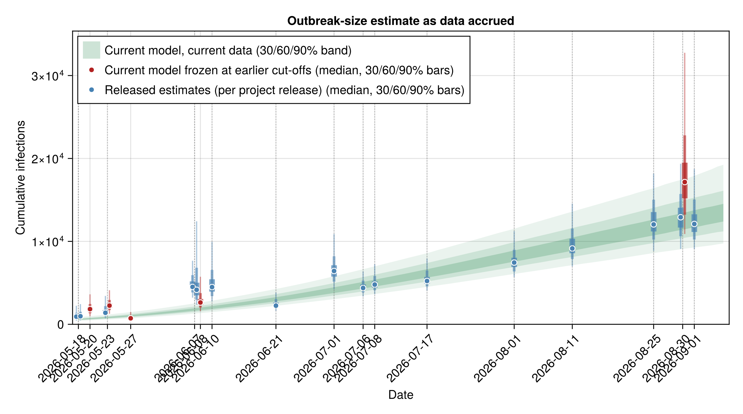
Reproduction number estimated by each data stream
The reproduction number each stream implies on its own, one panel per stream with the joint fit overlaid in grey as the reference.
Per-stream implied-Rt plot
# The per-stream fits walk Rt from day 1 (the default `rt_start`), while the
# joint walks from `RT_WALK_LEAD` days before the first situation report; the
# shared `display_start` is the joint renewal start so every stream reads over
# the same established window. `ramp` matches the joint Rt figure.
_rt_walk_start_joint = clamp(_BREAKPOINT - RT_WALK_LEAD, _rt_start_plot, obs.n);
stream_rt_fig = plot_rt_streams(
    [
        (; label = "exports", chn = chn_exports, rt_start = 1,
            rt_walk_start = 1, colour = :seagreen),
        (; label = "deaths (DRC)", chn = chn_deaths, rt_start = 1,
            rt_walk_start = 1, colour = :firebrick),
        (; label = "cases (DRC)", chn = chn_cases, rt_start = 1,
            rt_walk_start = 1, colour = :steelblue),
        (; label = "confirmed (DRC)", chn = chn_confirmed, rt_start = 1,
            rt_walk_start = 1, colour = :goldenrod),
        (; label = "isolation (DRC)", chn = chn_treatment, rt_start = 1,
            rt_walk_start = 1, colour = :darkorange),
        (; label = "onsets (DRC)", chn = chn_onsets, rt_start = 1,
            rt_walk_start = 1, colour = :mediumpurple)];
    joint = (; label = "joint", chn = chn_joint, rt_start = _rt_start_plot,
        rt_walk_start = _rt_walk_start_joint),
    n = obs.n, breakpoint = _BREAKPOINT,
    as_of_date = string(obs.cutoff), seeding = obs.seeding,
    display_start = _rt_start_plot, ramp = RT_INTERVENTION_RAMP);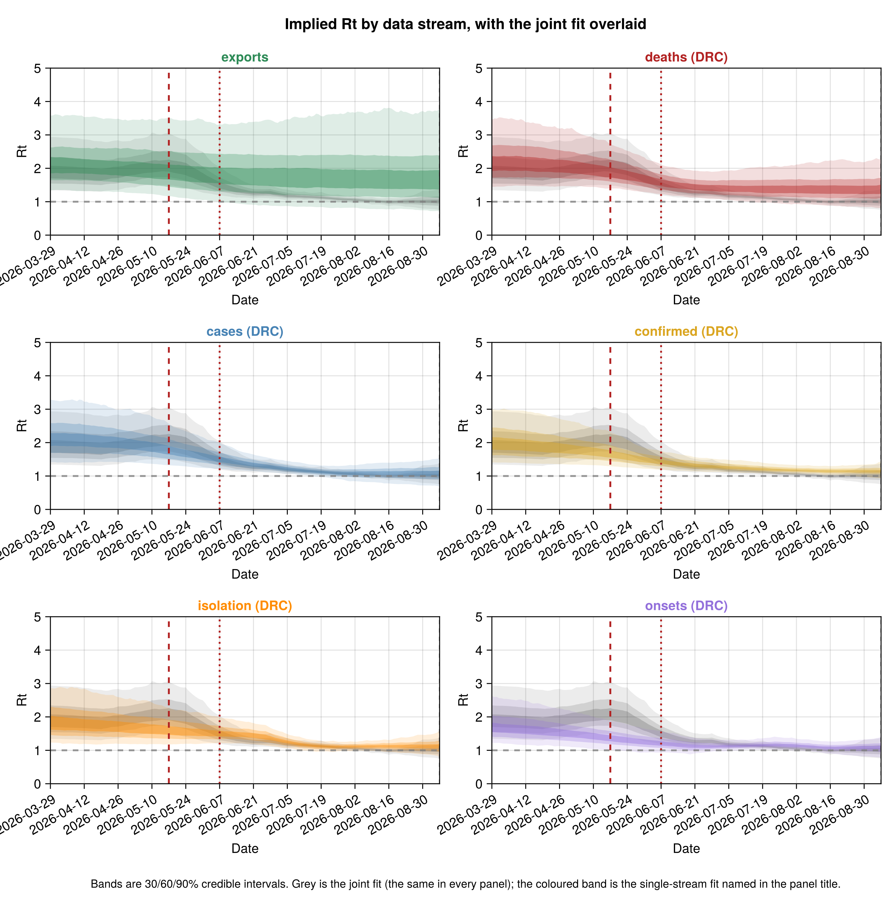
Reproduction number by release
The reproduction number estimated at each release, the same kind of release-by-release picture as the outbreak-size evolution above. Each release's cut-off reproduction number
Reproduction number per release with the current-fit band
rt_release_df = CSV.read(
    joinpath(pkgdir(BVDOutbreakSize), "data", "rt_by_release.csv"), DataFrame)
rt_release = [(string(r.date), r.median, r.lo30, r.hi30, r.lo60, r.hi60,
                  r.lo90, r.hi90) for r in eachrow(rt_release_df)]

# The current fit's daily Rt over its established window, summarised per day
# into a 30/60/90% band, reusing the same walk reconstruction the Rt figure
# uses so the band lines up with the per-release points on the calendar axis.
# The band is drawn only from the first release date onward, so it spans the
# same window as the per-release estimates rather than extending back to the
# renewal start. The first release day is the earliest date in
# `rt_by_release.csv` as a grid day; the walk is still reconstructed from the
# renewal start `_rt_start_plot` (the model knot grid) and the window is
# clamped into the reconstructed range so the quantiles never hit masked days.
rt_release_trajectory = let
    rt_walk_start = clamp(_BREAKPOINT - RT_WALK_LEAD, _rt_start_plot, obs.n)
    mat = reconstruct_rt(chn_joint; n = obs.n, breakpoint = _BREAKPOINT,
        rt_start = _rt_start_plot, rt_walk_start = rt_walk_start,
        ramp = RT_INTERVENTION_RAMP)
    first_release_day = clamp(
        value(minimum(rt_release_df.date) - obs.seeding) + 1,
        _rt_start_plot, obs.n)
    days = first_release_day:obs.n
    dates = [obs.seeding + Day(d - 1) for d in days]
    q(d, p) = quantile(collect(skipmissing(@view mat[:, d])), p)
    (dates,
        [q(d, 0.35) for d in days], [q(d, 0.65) for d in days],
        [q(d, 0.20) for d in days], [q(d, 0.80) for d in days],
        [q(d, 0.05) for d in days], [q(d, 0.95) for d in days])
end

rt_evolution_fig = plot_estimate_evolution(rt_release;
    trajectory = rt_release_trajectory,
    ylabel = "Reproduction number",
    title = "Reproduction number as data accrued",
    released_label = "Released estimate (per project release)",
    trajectory_label = "Current model, current data",
    refline = 1.0);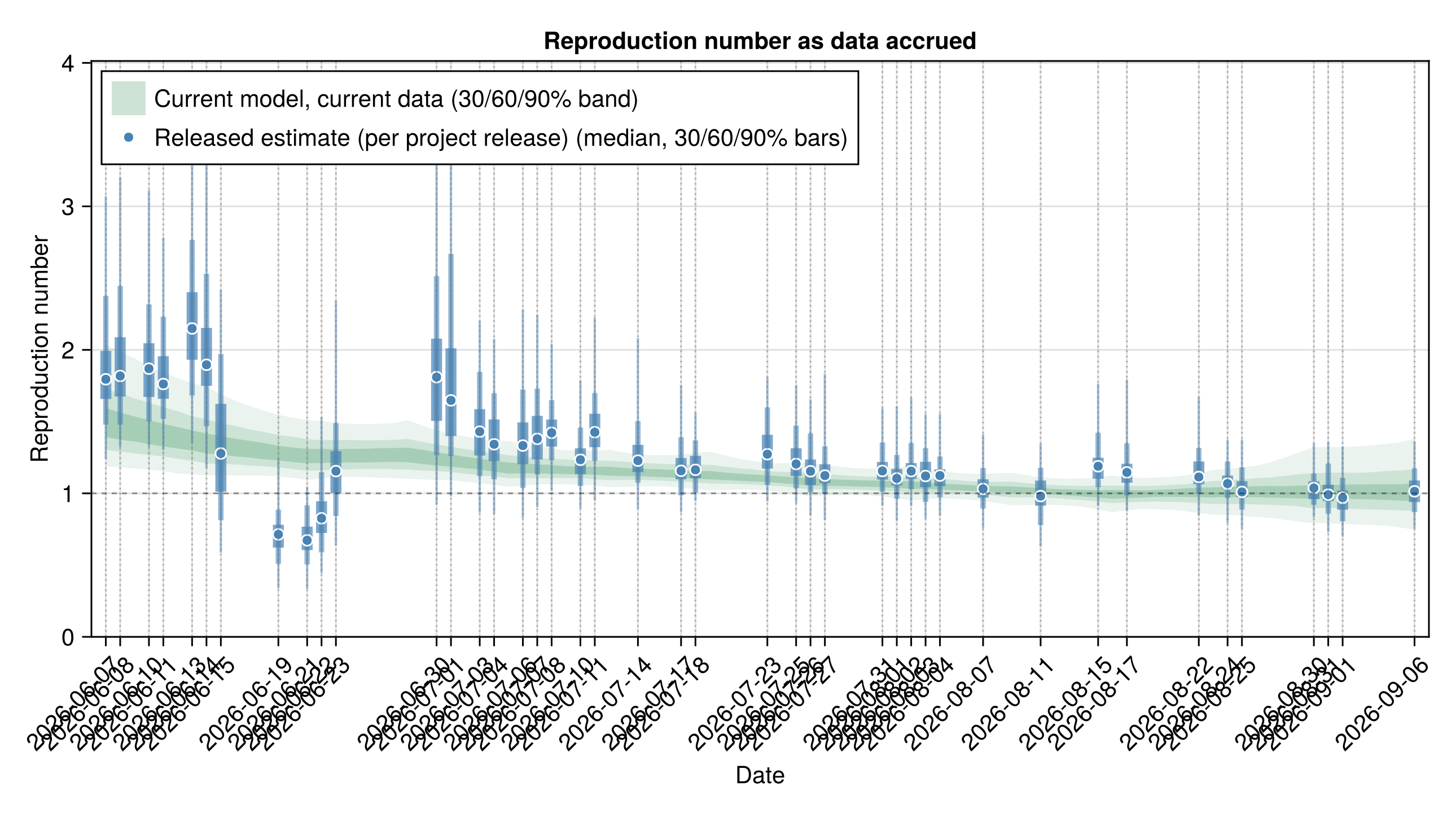
Reproduction number by release and dataset
The same release-by-release reproduction number split into one panel per dataset, so each dataset's history reads against the others and against the joint. Panels share a calendar axis and a y range, and
Reproduction number per release by fit
# Schema of the per-release, per-fit estimate tables written by
# scripts/score_releases.jl from each release's stream_estimates.csv.
_by_stream_schema = (; release = String, date = Date, fit = String,
    median = Float64, lo30 = Float64, hi30 = Float64, lo60 = Float64,
    hi60 = Float64, lo90 = Float64, hi90 = Float64)

# Fits in a fixed order, the joint first, so the panels do not reshuffle
# between builds. Labels match the per-stream table above (in "Outbreak
# size estimated by each data stream"). Recovered is absent because it
# has no individual fit.
_fit_order = ["joint", "cases", "deaths", "confirmed", "confirmed_deaths",
    "treatment", "onsets", "exports"]
_fit_labels = Dict("joint" => "joint", "cases" => "cases (DRC)",
    "deaths" => "deaths (DRC)", "confirmed" => "confirmed (DRC)",
    "confirmed_deaths" => "confirmed deaths (DRC)",
    "treatment" => "isolation (DRC)", "onsets" => "onsets (DRC)",
    "exports" => "exports")

# Group a per-fit estimate table into the label => tuples pairs the faceted
# plot takes, keyed on the date so the mixed release tag shapes
# (`results-v1.9.0` and `results-1243`) never reach the axis.
function _fit_groups(df)
    return [get(_fit_labels, f, f) =>
                [(string(r.date), r.median, r.lo30, r.hi30, r.lo60, r.hi60,
                     r.lo90, r.hi90) for r in eachrow(df) if r.fit == f]
            for f in _fit_order]
end

# Per-fit reproduction-number trajectory, reconstructing the walk exactly as
# `plot_rt_streams` does per stream.
function _stream_rt_trajectory(chn, dates; rt_start, rt_walk_start)
    mat = reconstruct_rt(chn; n = obs.n, breakpoint = _BREAKPOINT,
        rt_start = rt_start, rt_walk_start = rt_walk_start,
        ramp = RT_INTERVENTION_RAMP)
    first_date = isempty(dates) ? obs.seeding : minimum(dates)
    first_day = clamp(value(first_date - obs.seeding) + 1, rt_start, obs.n)
    days = first_day:obs.n
    ds = [obs.seeding + Day(d - 1) for d in days]
    q(d, p) = quantile(collect(skipmissing(@view mat[:, d])), p)
    (ds,
        [q(d, 0.35) for d in days], [q(d, 0.65) for d in days],
        [q(d, 0.20) for d in days], [q(d, 0.80) for d in days],
        [q(d, 0.05) for d in days], [q(d, 0.95) for d in days])
end

# The single-stream chains and their renewal-walk starts, keyed on the fit
# id the per-release tables use. Both the joint walk start and the day-1
# per-stream starts are the ones the per-stream implied-Rt figure above
# uses, so the bands here match it. Confirmed deaths has no trajectory
# here: its panel still draws its release points alone.
_stream_chains = (
    "joint" => (; chn = chn_joint, rt_start = _rt_start_plot,
        rt_walk_start = _rt_walk_start_joint),
    "cases" => (; chn = chn_cases, rt_start = 1, rt_walk_start = 1),
    "deaths" => (; chn = chn_deaths, rt_start = 1, rt_walk_start = 1),
    "confirmed" => (; chn = chn_confirmed, rt_start = 1, rt_walk_start = 1),
    "treatment" => (; chn = chn_treatment, rt_start = 1, rt_walk_start = 1),
    "onsets" => (; chn = chn_onsets, rt_start = 1, rt_walk_start = 1),
    "exports" => (; chn = chn_exports, rt_start = 1, rt_walk_start = 1))

# Build a fit label => trajectory dictionary from a per-release table,
# restricted to the fits `_stream_chains` names. A fit with no row in `df`
# gets no trajectory, so its panel still draws its release points alone.
function _rt_trajectories(df)
    trajs = Dict{String, Any}()
    for (fid, cfg) in _stream_chains
        fdates = df.date[df.fit .== fid]
        isempty(fdates) && continue
        trajs[get(_fit_labels, fid, fid)] = _stream_rt_trajectory(
            cfg.chn, fdates; rt_start = cfg.rt_start,
            rt_walk_start = cfg.rt_walk_start)
    end
    return trajs
end

rt_stream_df = _release_data("rt_by_release_by_stream.csv",
    _by_stream_schema)
rt_stream_fig = plot_evolution_by_group(_fit_groups(rt_stream_df);
    trajectories = _rt_trajectories(rt_stream_df),
    ylabel = "Reproduction number",
    title = "Reproduction number as data accrued, by dataset",
    released_label = "Released estimate (per release)",
    refline = 1.0,
    empty_note = "No per-dataset reproduction numbers saved yet.");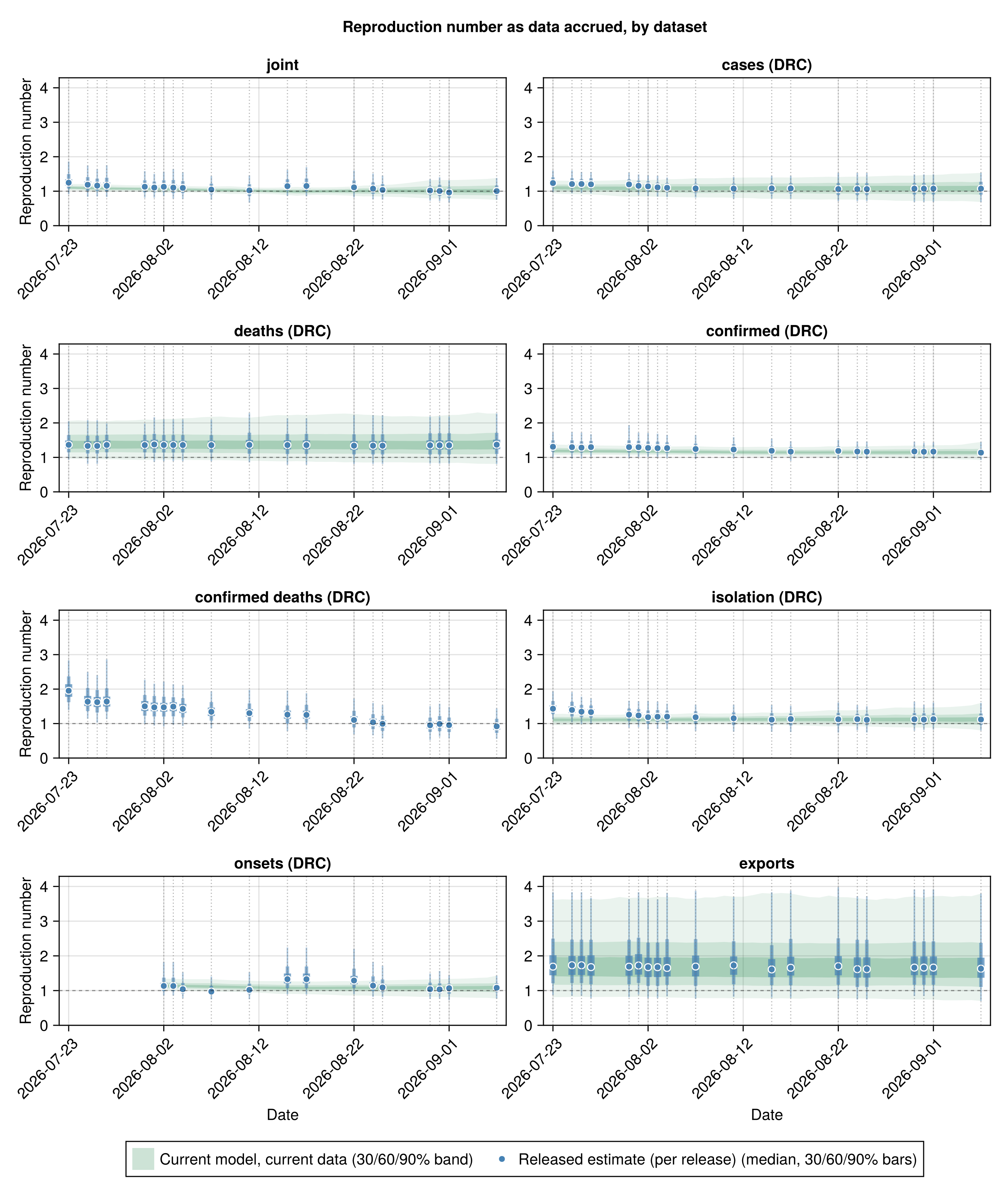
Basic reproduction number by release
The basic reproduction number
Basic reproduction number per release with frozen re-fits and the current-fit band
# Per-release R0 points from r0_by_release.csv, read through the typed
# fallback so a missing or header-only file (until a release carries
# `rt_state.log_R0` in its posterior draws) does not break the build. The
# schema mirrors rt_by_release.csv.
_r0_schema = (; release = String, date = Date, median = Float64,
    lo30 = Float64, hi30 = Float64, lo60 = Float64, hi60 = Float64,
    lo90 = Float64, hi90 = Float64)
r0_release_df = _release_data("r0_by_release.csv", _r0_schema)
r0_release = [(string(r.date), r.median, r.lo30, r.hi30, r.lo60, r.hi60,
                  r.lo90, r.hi90) for r in eachrow(r0_release_df)]

# The current model frozen at earlier cut-offs, one discrete estimate per
# cut-off, reusing the same frozen fits `frozen_matched` above already
# computed. No extra fits are run. Each tuple carries the median and
# 30/60/90% credible bounds of that frozen fit's own R0 draws, unrounded
# since R0 is continuous.
frozen_r0_matched = [(c, _ci369(frozen_R0(c); round_fn = identity)...)
                     for c in _frozen_matched_cutoffs]

# The current fit's R0 posterior is a single distribution rather than a
# daily series, so it summarises into a flat 30/60/90% reference band. The
# window runs from the earliest mark on the axis, the first frozen cut-off
# or release point, to the current cut-off, so the band reads behind both
# series rather than only their recent end.
r0_reference = let
    draws = r0_walk_draws(chn_joint)
    q(p) = quantile(draws, p)
    first_date = min(minimum(Date.(_frozen_matched_cutoffs)),
        isempty(r0_release_df.date) ? obs.cutoff :
        minimum(r0_release_df.date))
    dates = [first_date, obs.cutoff]
    (dates, fill(q(0.35), 2), fill(q(0.65), 2), fill(q(0.20), 2),
        fill(q(0.80), 2), fill(q(0.05), 2), fill(q(0.95), 2))
end

r0_evolution_fig = plot_estimate_evolution(r0_release;
    renewal = frozen_r0_matched,
    renewal_label = "Current model frozen at earlier cut-offs",
    trajectory = r0_reference,
    ylabel = "Basic reproduction number",
    title = "Basic reproduction number as data accrued",
    released_label = "Released estimate (per project release)",
    trajectory_label = "Current model, current data",
    refline = 1.0);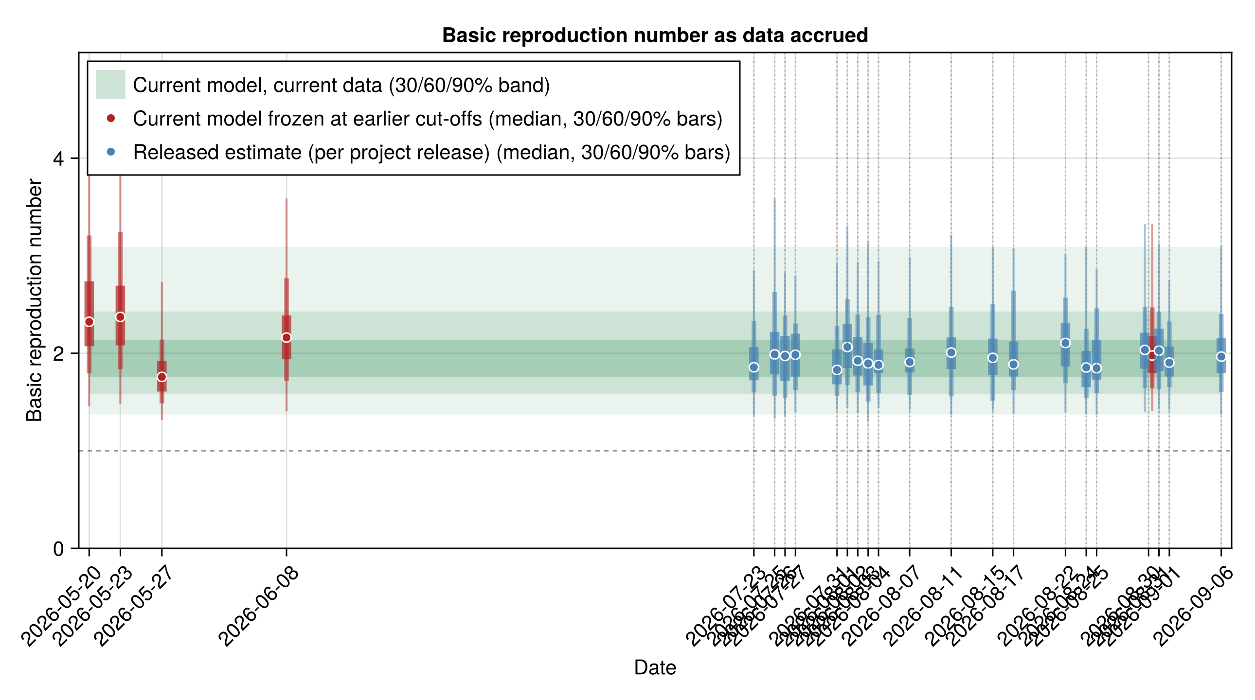
Basic reproduction number by release and dataset
The basic reproduction number estimated at each release, one panel per fit, the by-dataset counterpart of the figure above. Panels share a calendar axis and a y range, and
Basic reproduction number per release by fit
# Per-fit R0 flat reference band, the by-dataset counterpart of
# `r0_reference` above, a single distribution rather than a daily walk, so
# each fit's band is flat across its own release window. `r0_walk_draws`
# probes for the walk base, so a single-stream model built without its own
# renewal walk drops its band instead of erroring.
function _r0_stream_trajectory(chn, dates)
    draws = r0_walk_draws(chn)
    isnothing(draws) && return nothing
    q(p) = quantile(draws, p)
    first_date = isempty(dates) ? obs.seeding : minimum(dates)
    ds = [first_date, obs.cutoff]
    (ds, fill(q(0.35), 2), fill(q(0.65), 2), fill(q(0.20), 2),
        fill(q(0.80), 2), fill(q(0.05), 2), fill(q(0.95), 2))
end

# Build a fit label => trajectory dictionary from a per-release R0 table,
# restricted to the fits `_stream_chains` names, the same restriction the
# reproduction-number-by-dataset trajectories use. A fit with no row in
# `df`, or whose chain carries no walk base, gets no trajectory, so its
# panel still draws its release points alone.
function _r0_trajectories(df)
    trajs = Dict{String, Any}()
    for (fid, cfg) in _stream_chains
        fdates = df.date[df.fit .== fid]
        isempty(fdates) && continue
        traj = _r0_stream_trajectory(cfg.chn, fdates)
        isnothing(traj) || (trajs[get(_fit_labels, fid, fid)] = traj)
    end
    return trajs
end

r0_stream_df = _release_data("r0_by_release_by_stream.csv",
    _by_stream_schema)
r0_stream_fig = plot_evolution_by_group(_fit_groups(r0_stream_df);
    trajectories = _r0_trajectories(r0_stream_df),
    ylabel = "Basic reproduction number",
    title = "Basic reproduction number as data accrued, by dataset",
    released_label = "Released estimate (per release)",
    refline = 1.0,
    empty_note = "No per-dataset basic reproduction numbers saved yet.");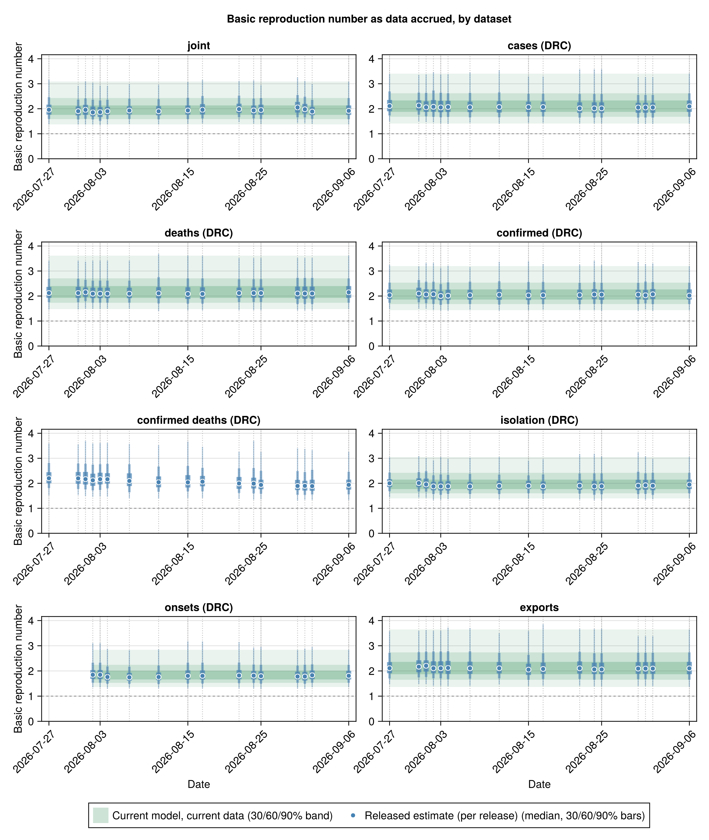
Comparison with McCabe et al.
Our model is a discrete-time renewal model with a time-varying reproduction number and every data stream fitted jointly. McCabe et al. published their estimates as scenarios at fixed situation-report cut-offs, each scenario carrying a 95% confidence interval. We show all three, the 18 May report, the 20 May update and the 27 May Lancet publication, as one panel each, with their intervals kept. Within a panel each method and scenario family is a single line, carrying its sweep over the nuisance assumptions: the case-fatality ratio, the geographic window and the doubling time. The geographic-spread scenarios come from exported cases and travel volume. Their back-calculation-from-deaths scenarios differ between the reports, since the 18 May report used 88 reported deaths and the 20 May update 131. The 20 May update also corrected the case-fatality ratios. McCabe's scenarios estimate cumulative cases at their report dates, though their report is not fully explicit about whether this is symptomatic cases or all infections. We take the like-for-like quantity to be our cumulative symptom onsets on the same dates, not the latent infections (which include the not-yet-symptomatic) or our current cut-off total. We read our value off the joint fit's cumulative-onset trajectory at the grid day for each report date, and show it with its credible interval. Each scenario sits beside our estimate for the date it was made: the 18 May report against our 18 May value, the 20 May update against our 20 May value, and the 27 May Lancet publication against our 27 May value.
McCabe scenarios with uncertainty against our estimates
function _ci90row(xs)
    (round(Int, quantile(xs, 0.5)),
        round(Int, quantile(xs, 0.05)),
        round(Int, quantile(xs, 0.95)))
end

# Our modelled cumulative symptom onsets on a McCabe report date, read off
# the joint fit's per-draw `cumulative_onsets` trajectory. The grid runs to
# the cut-off on day `n`, so the day-index for a date is `n` minus the days
# from that date back to the cut-off (`grid_day("2026-06-07") = n`,
# `"2026-05-20") = n - 18`, `"2026-05-18") = n - 20`).
_onset_trajs = let mat = chn_joint[:cumulative_onsets]
    [collect(v) for v in vec(collect(mat))]
end
# Inverse of `grid_date(day) = obs.cutoff - Day(obs.n - day)`: the day-index
# whose calendar date is `date`, using `value` (imported above) for the
# day count rather than the non-exported `Dates.date2epochdays`.
_grid_day(date) = obs.n - value(obs.cutoff - Date(date))
function _ours_on(date)
    d = _grid_day(date)
    _ci90row(Float64[t[d] for t in _onset_trajs])
end

# Our matched cumulative-onset estimate for each report date, keyed by date so
# it lands beside that vintage's scenarios in its own panel.
mccabe_ours = Dict(
    "2026-05-18" => _ours_on("2026-05-18"),
    "2026-05-20" => _ours_on("2026-05-20"),
    "2026-05-27" => _ours_on("2026-05-27"))

# One panel per report date; within a panel each method-and-family is one row,
# with the case-fatality / window / doubling-time sweep dodged onto that single
# line, so the ~40 scenarios keep their intervals without becoming ~40 rows.
matched_comparison_fig = plot_scenario_comparison(REPORT_SCENARIOS_CI;
    ours = mccabe_ours,
    date_titles = ["2026-05-18" => "18 May report",
        "2026-05-20" => "20 May update",
        "2026-05-27" => "27 May (Lancet)"],
    xlabel = "Cumulative cases");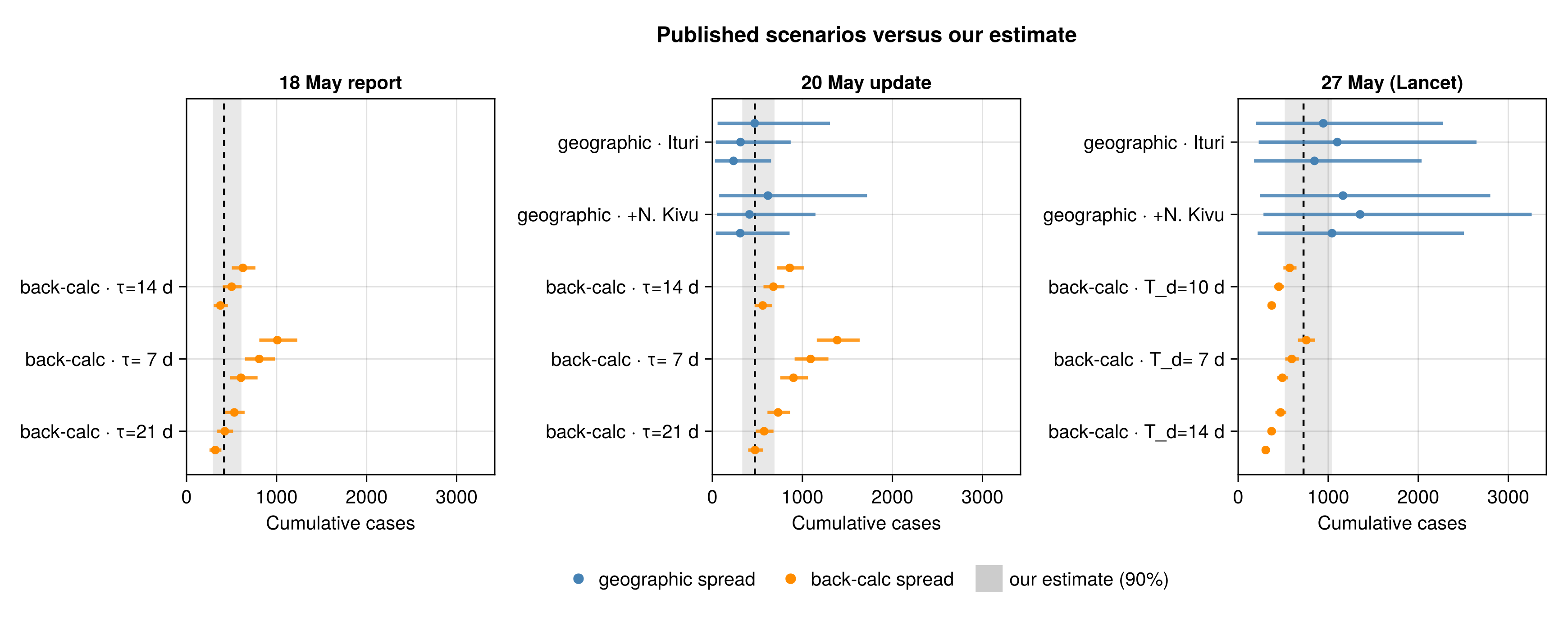
The McCabe scenarios are outbreak-size estimates, the same quantity our renewal model and the released integral model report. Their 95% confidence intervals come from exact negative-binomial counts for the geographic-spread method and a Poisson likelihood profile for the back-calculation from deaths.
Frozen-fit C_T intervals (kept for the CSV export, not shown)
# The estimate-evolution figure above already shows how the size estimate
# shifts as data accrues, so the side-by-side frozen-fit table is no longer
# rendered in the report; it is kept only to populate the published
# `frozen_matched_cutoffs.csv` export.
frozen_streams_table = streams_table(
    "frozen 20 May" => frozen_C("2026-05-20"),
    "frozen 23 May" => frozen_C("2026-05-23"),
    "frozen 27 May" => frozen_C("2026-05-27"),
    "frozen 8 June" => frozen_C(default_chamla_cutoff()),
    "current data" => posterior_C_joint);
Comparison with Chamla et al.
A second group, Chamla et al. (Chamla et al., 2026) at the World Health Organization Regional Office for Africa, published a stochastic compartmental model of the same outbreak on 25 June 2026. Their model is a discrete-time susceptible-exposed-infectious-recovered-dead ensemble, recalibrated by simulation filtering to the laboratory-confirmed case series and anchored on the 598 confirmed cases reported by 8 June. It is then run forward to project the confirmed-case trajectory under a low, central and high transmissibility scenario.
Their published quantity is the cumulative confirmed-case count, with the reporting fraction held at one, so it does not adjust for the cases that are infected but never laboratory-confirmed. This is a different quantity from the cumulative cases this analysis and McCabe et al. estimate, which include the unconfirmed and unascertained. It therefore sits below them: a floor on the true size rather than an estimate of it. The like-for-like comparison is therefore against our own confirmed-case projection, not against our cumulative infection count.
We compare forward projections rather than refitting to their assumptions. We take our fit frozen at 8 June, the exact date of their confirmed-case calibration anchor. We roll its confirmed-case stream forward to the dates Chamla report, using the same machinery as the one-week-ahead forecast. Setting our projection, their projection and the confirmed cases observed since on one timeline shows how each projection has held up against the data.
Project the 8 June fit forward and assemble the Chamla comparison
# The 8 June frozen joint fit matches Chamla's confirmed-case calibration
# anchor exactly and carries the confirmed-case testing history through then,
# so we roll its confirmed-case stream forward with the one-week-ahead forecast
# machinery to the dates Chamla report.
chamla_anchor = frozen_by_cutoff["2026-06-08"]

# Our projected cumulative confirmed cases at a horizon of `h` days past the
# 8 June cut-off: a forward `forecast_reported` run (its reproduction number
# left to keep evolving), summarised as (median, 5%, 95%).
function _our_confirmed_h(h)
    fc = forecast_reported(chamla_anchor.chn;
        horizon = h,
        obs_cases = chamla_anchor.o.reported_cases,
        obs_deaths = chamla_anchor.o.total_deaths,
        obs_confirmed = chamla_anchor.o.confirmed_cases,
        obs_confirmed_deaths = chamla_anchor.o.confirmed_deaths)
    return _ci90row(float.(fc.confirmed_cum))
end

# Our projection at Chamla's forward report dates (10 and 24 June, week 12):
# the anchor day is the fitted confirmed total at 8 June, each later date a
# forward forecast. Reused for the matched-date table and the week-12 figure.
chamla_fan = map(["2026-06-08", "2026-06-10", "2026-06-24"]) do d
    h = value(Date(d) - chamla_anchor.cutoff)
    row = h == 0 ?
          (chamla_anchor.o.confirmed_cases, chamla_anchor.o.confirmed_cases,
        chamla_anchor.o.confirmed_cases) : _our_confirmed_h(h)
    (d, row...)
end
_fan_at(date) =
    let r = first(x for x in chamla_fan if x[1] == date)
        (r[2], r[3], r[4])
    end
ours_10jun = _fan_at("2026-06-10")
ours_24jun = _fan_at("2026-06-24")

# Observed confirmed cases over the comparison window: the daily cumulative
# series read off the chain's grid from 18 May (Chamla's first projected point)
# to the cut-off.
chamla_obs_series = let
    ds = [grid_date(d) for d in obs.confirmed_history.days]
    cs = obs.confirmed_history.counts
    [(string(ds[i]), cs[i]) for i in eachindex(ds) if ds[i] >= Date("2026-05-18")]
end

# Chamla's central confirmed-case projection over the comparison window; their
# later, far-larger horizons are noted in the text rather than plotted so the
# window stays legible.
chamla_central_window = CHAMLA_CONFIRMED_CENTRAL[1:4]

chamla_projection_fig = plot_projection_comparison(;
    external = chamla_central_window,
    ours = chamla_fan,
    observed = chamla_obs_series,
    external_label = "Chamla et al. central (R₀=1.71)",
    ours_label = "Our projection (from 8 June)",
    observed_label = "Observed confirmed",
    title = "Confirmed-case projections versus observed, from mid-May");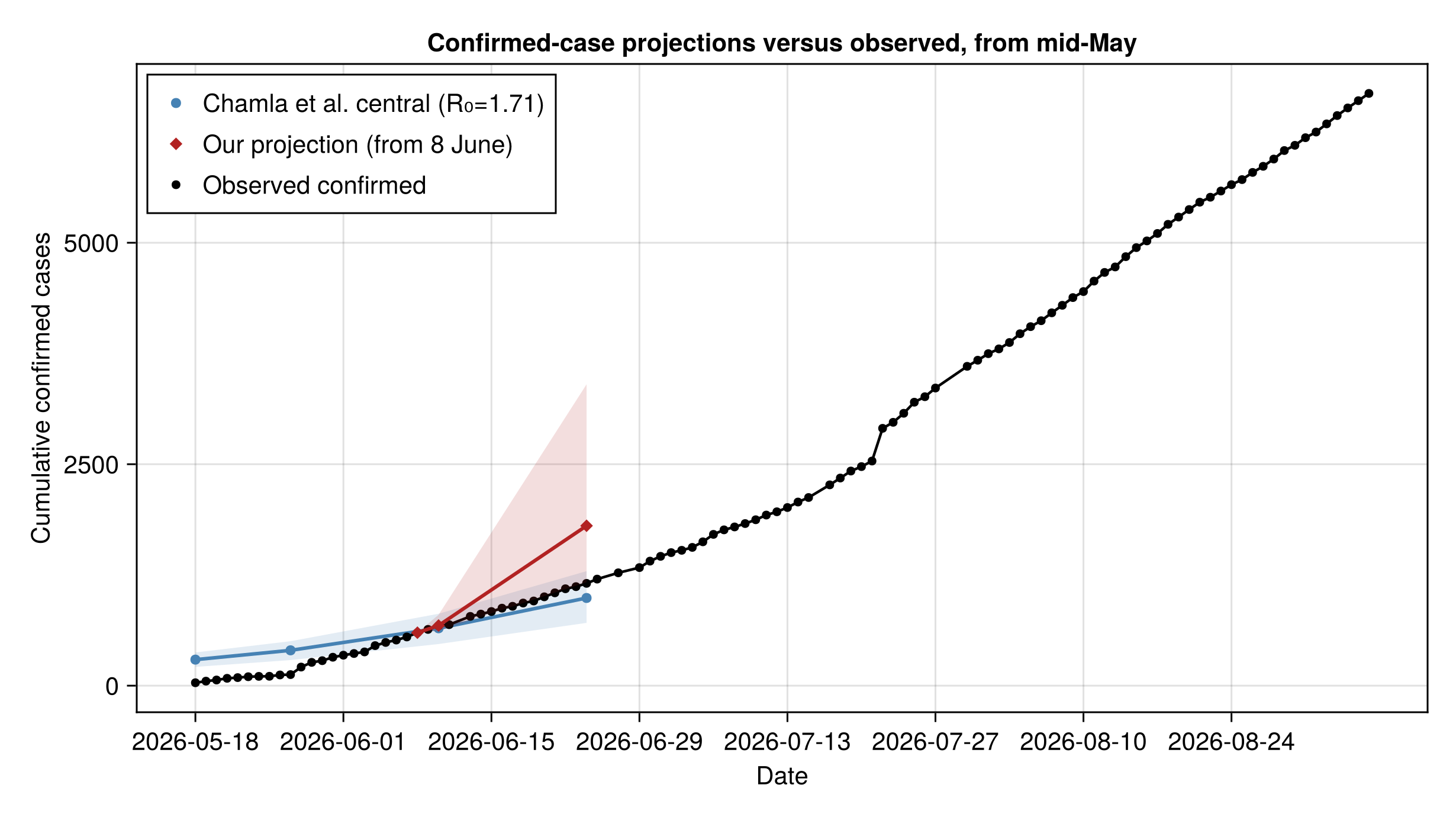
By 24 June their central scenario projected just under a thousand confirmed cases, and their low and high scenarios ranged from roughly 870 to 1360. The figure below sets that week-12 scenario spread beside our 8 June projection for the same date and the confirmed count observed by the cut-off, so each reads against their three scenarios at a glance.
Week-12 (24 June) scenario spread against ours and observed
chamla_w12_rows = vcat(
    [(label, m, lo, hi) for (label, m, lo, hi) in CHAMLA_CONFIRMED_W12],
    [("Our projection (from 8 June)", ours_24jun...)],
    [("Observed by 23 June cut-off", obs.confirmed_cases,
        obs.confirmed_cases, obs.confirmed_cases)])
chamla_w12_groups = vcat(fill("Chamla et al. scenarios", 3),
    ["Our projection"], ["Observed"])

chamla_w12_fig = plot_estimate_comparison(chamla_w12_rows;
    xlabel = "Cumulative confirmed cases by 24 June",
    groups = chamla_w12_groups,
    group_colours = ["Chamla et al. scenarios" => :steelblue,
        "Our projection" => :firebrick,
        "Observed" => :black]);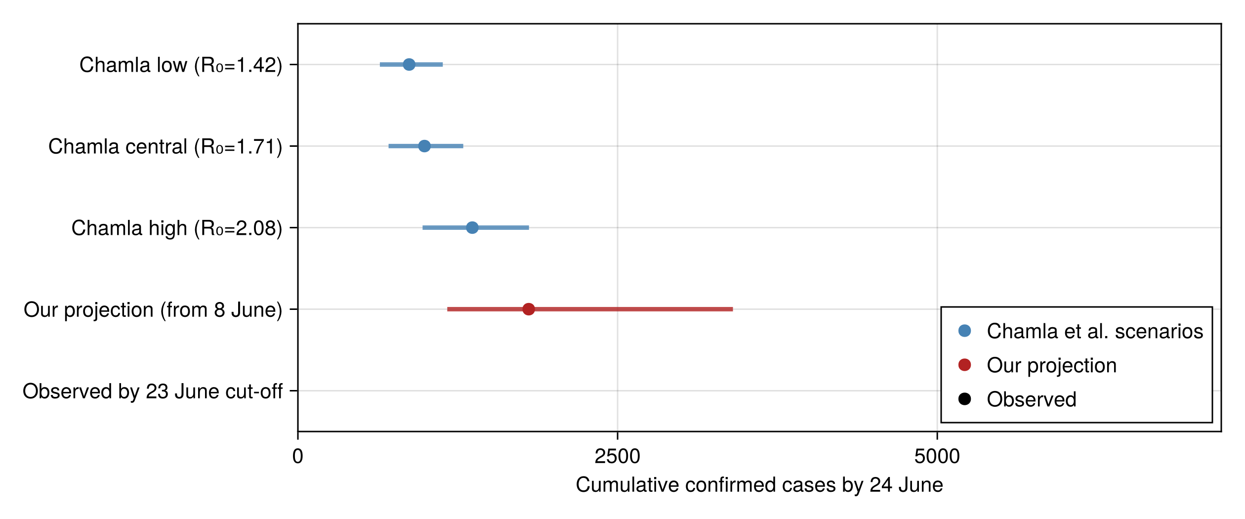
The matched-date numbers behind these figures are in the dropdown below, with the observed column taken to the 23 June cut-off.
Matched-date projection numbers (10 and 24 June)
chamla_comparison_table = let
    fmt(t) = string(t[1], " (", t[2], "–", t[3], ")")
    central(date) =
        let r = first(x for x in CHAMLA_CONFIRMED_CENTRAL
            if x[1] == date)
            fmt((r[2], r[3], r[4]))
        end
    DataFrame(
        "Date" => ["10 June", "24 June"],
        "Chamla central (90% PI)" => [central("2026-06-10"),
            central("2026-06-24")],
        "Our projection (90% CrI)" => [fmt(ours_10jun), fmt(ours_24jun)],
        "Observed confirmed" => [
            string(freeze_observations("2026-06-10").confirmed_cases),
            string(obs.confirmed_cases) * " (23 June)"])
end;| Date | Chamla central (90% PI) | Our projection (90% CrI) | Observed confirmed |
|---|---|---|---|
| 10 June | 648 (470–812) | 679 (619–800) | 676 |
| 24 June | 990 (709–1293) | 1805 (1168–3402) | 6686 (23 June) |
Beyond the comparison window their central scenario continues to roughly 8200 confirmed cases by mid-September, with the high scenario far higher. Those longer projections are not set against data here.
Reproduction number behind the projection
The forward projection above is carried by the reproduction-number trajectory our 8 June fit estimated, a quantity we report in its own right rather than as a comparison. The figure shows that trajectory, the time-varying reproduction number from the renewal walk with its credible intervals, as the fit saw it at 8 June. It declines over the weeks leading to the cut-off, and that decline is what bends the projected trajectory away from sustained early growth.
Reproduction number as estimated by the 8 June fit
# Reconstruct the reproduction-number trajectory the 8 June fit estimated,
# mirroring the current-data R_t figure but with the frozen vintage's own grid,
# breakpoint and renewal start.
chamla_rt_obs = chamla_anchor.o
chamla_rt_breakpoint = chamla_rt_obs.n - chamla_rt_obs.who_first_sitrep_days
chamla_rt_start = clamp(
    chamla_rt_obs.n - round(Int, chamla_rt_obs.tmrca_days) + RENEWAL_START_LEAD,
    1, chamla_rt_obs.n)
chamla_rt_fig = plot_rt(chamla_anchor.chn;
    n = chamla_rt_obs.n, breakpoint = chamla_rt_breakpoint,
    rt_start = chamla_rt_start,
    rt_walk_start = clamp(chamla_rt_breakpoint - RT_WALK_LEAD,
        chamla_rt_start, chamla_rt_obs.n),
    as_of_date = string(chamla_rt_obs.cutoff),
    seeding = chamla_rt_obs.seeding, ramp = RT_INTERVENTION_RAMP);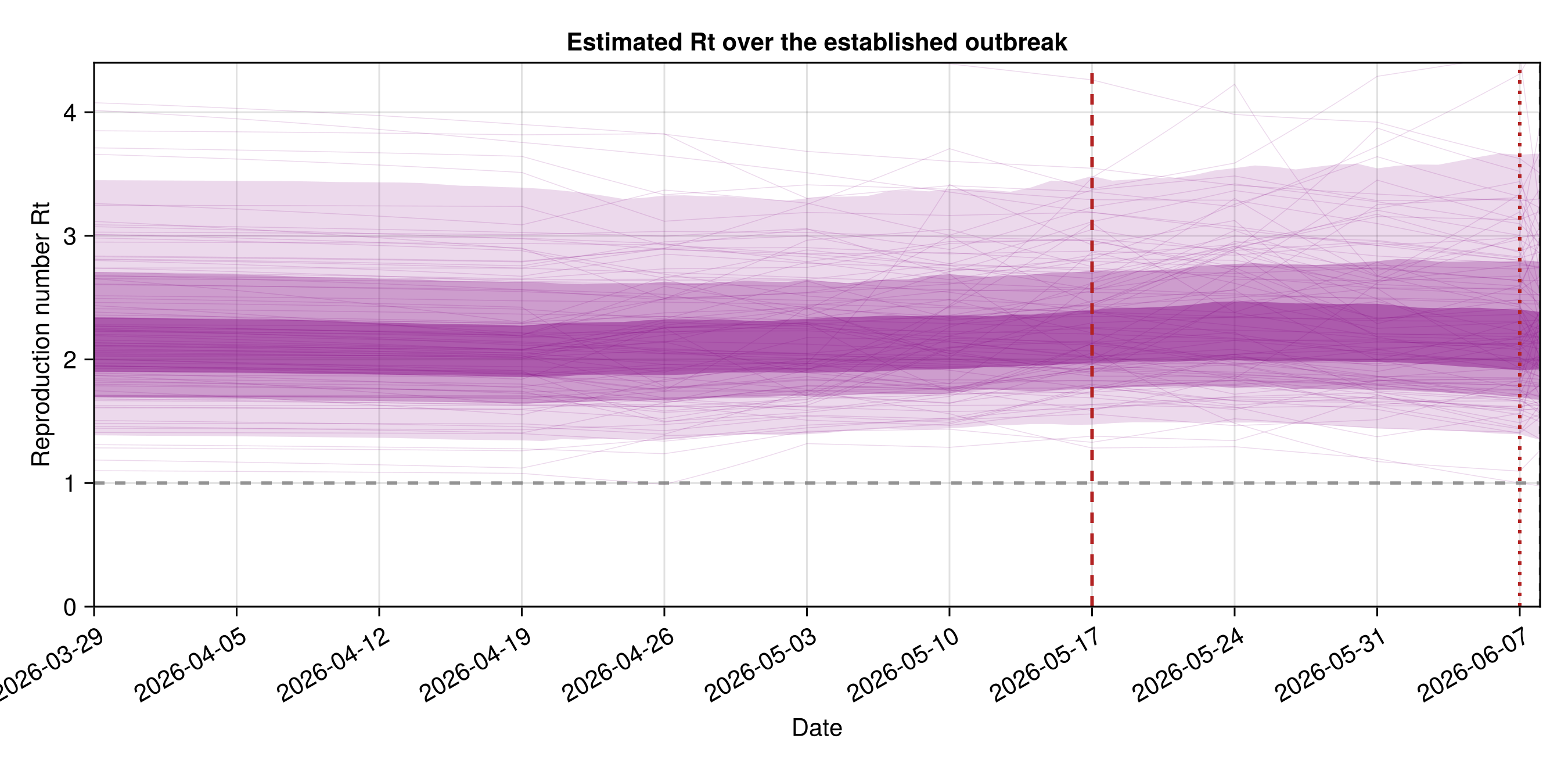
Delay sensitivity
The death stream dates the outbreak from how far deaths lag symptom onset, so the assumed onset-to-death delay sets the implied infection count. The baseline uses the hospital-pathway delay from the Isiro 2012 line-list reanalysis (onset to admission then admission to death, implied mean about 12 d). We re-fit the joint model under the community-pathway delay from the same reanalysis: the delay for deaths that occur in the community without a recorded admission. This delay is shorter (implied mean about 8 d). Both pathways come from the line list, so this varies the actual delay assumption rather than an arbitrary scenario. The re-fit uses the full headline settings: 1000 draws across two chains.
The infection count to date shifts with the assumed delay, and the table and overlaid densities below show how far.
Re-fit the joint under the community-pathway onset-to-death delay
# The sensitivity re-fits (community-delay variant) are
# defined in the fit registry (`docs/fits/registry.jl`) and loaded through the cache
# (when enabled) in the setup block above.
posterior_C_community_delay = RUN_SENSITIVITY ?
                              vec(Array(chn_joint_community_delay[:C_T])) : nothing;
Delay-sensitivity infection-count table
delay_sensitivity_table = RUN_SENSITIVITY ?
                          streams_table("baseline (hospital pathway)" => posterior_C_joint,
    "community pathway" => posterior_C_community_delay) :
Markdown.md"_Delay sensitivity analysis not shown in this build._";| Stream | Lower 90% | Lower 60% | Lower 30% | Upper 30% | Upper 60% | Upper 90% |
|---|---|---|---|---|---|---|
| baseline (hospital pathway) | 9749 | 11206 | 12399 | 14531 | 16111 | 19236 |
| community pathway | 10142 | 11451 | 12468 | 14829 | 16372 | 20370 |
Delay-sensitivity infection-count density plot
delay_sensitivity_fig = RUN_SENSITIVITY ?
                        plot_cumulative_cases(
    "baseline (hospital pathway)" => posterior_C_joint,
    "community pathway" => posterior_C_community_delay; scenarios = []) :
                        Markdown.md"_Delay sensitivity analysis not shown in this build._";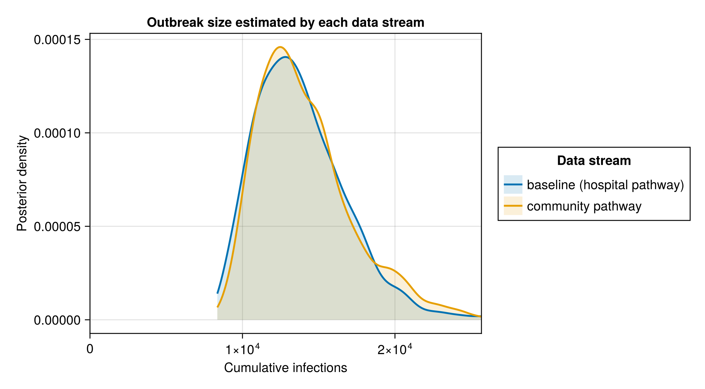
Tree-prior sensitivity
The outbreak-age estimate depends on the coalescent tree prior assumed in the BEAST X analysis. The baseline uses the more flexible Skygrid non-parametric model, which dates the common ancestor to 15 March 2026 (
Re-fit the joint under the Exponential growth tree prior
# The Exponential-growth re-fit (and its `tmrca_days` offset) is defined in the fit
# registry (`docs/fits/registry.jl`) and loaded through the cache (when enabled) in the
# setup block above.
posterior_C_exp_growth = RUN_SENSITIVITY ?
                         vec(Array(chn_joint_exp_growth_clock[:C_T])) : nothing
T_skygrid = vec(Array(chn_joint[:T]))
T_exp_growth = RUN_SENSITIVITY ? vec(Array(chn_joint_exp_growth_clock[:T])) : nothing;
The infection count to date under the two tree priors, side by side. A slightly earlier common ancestor (Exponential growth) permits a marginally older outbreak, though the difference is small because the evolutionary rates are nearly identical.
Tree-prior infection-count table
clock_sensitivity_C_table = RUN_SENSITIVITY ?
                            streams_table("Skygrid (baseline)" => posterior_C_joint,
    "Exponential growth" => posterior_C_exp_growth) :
Markdown.md"_Tree-prior sensitivity analysis not shown in this build._";| Stream | Lower 90% | Lower 60% | Lower 30% | Upper 30% | Upper 60% | Upper 90% |
|---|---|---|---|---|---|---|
| Skygrid (baseline) | 9749 | 11206 | 12399 | 14531 | 16111 | 19236 |
| Exponential growth | 9968 | 11172 | 12214 | 14299 | 15665 | 18503 |
Tree-prior infection-count density plot
clock_sensitivity_C_fig = RUN_SENSITIVITY ?
                          plot_cumulative_cases("Skygrid (baseline)" => posterior_C_joint,
    "Exponential growth" => posterior_C_exp_growth; scenarios = []) :
                          Markdown.md"_Tree-prior sensitivity analysis not shown in this build._";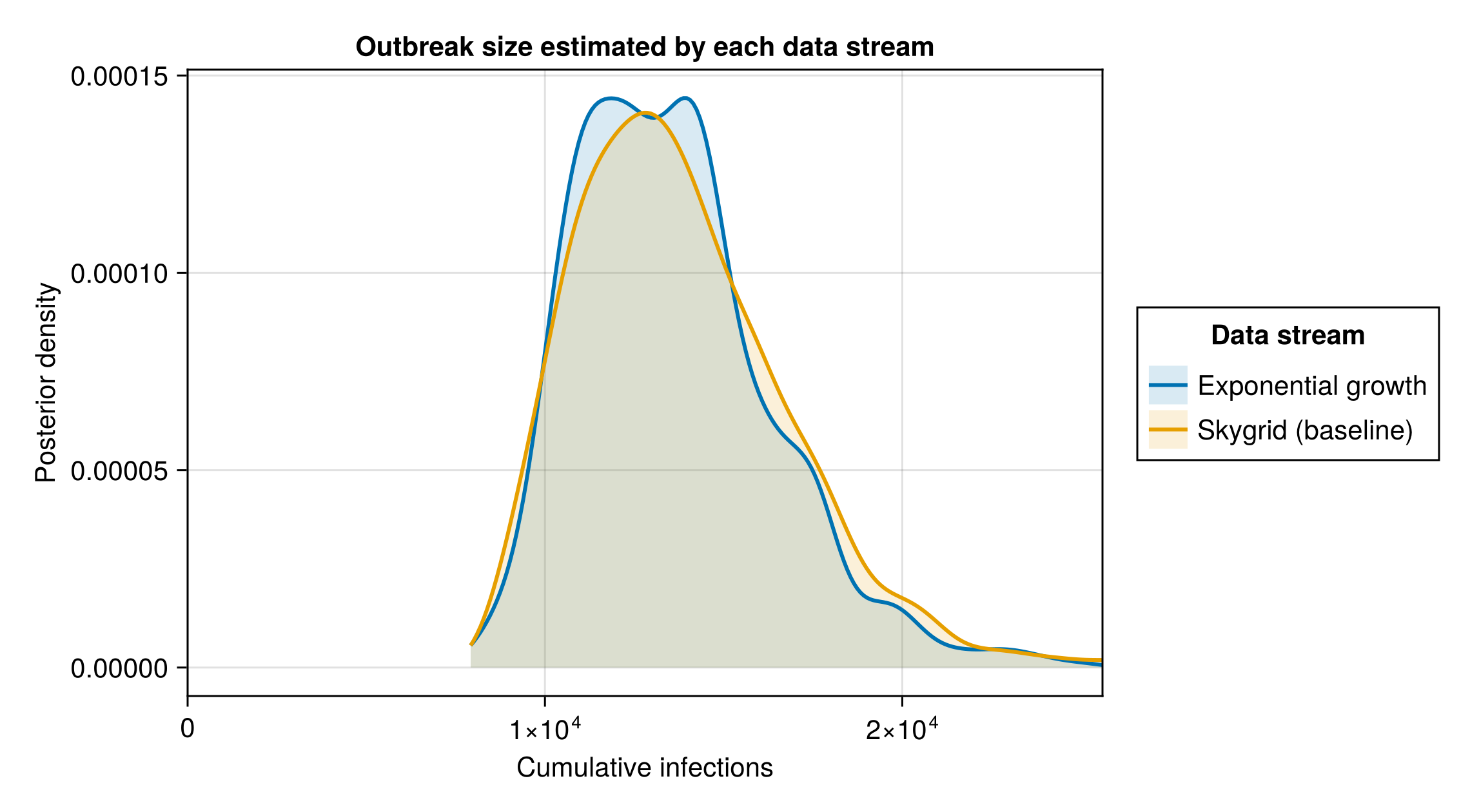
The outbreak age, the number of days from seeding to the cut-off, under the two tree priors.
Tree-prior outbreak-age table
clock_sensitivity_T_table = RUN_SENSITIVITY ?
                            streams_table("Skygrid (baseline)" => T_skygrid,
    "Exponential growth" => T_exp_growth; digits = 0) :
Markdown.md"_Tree-prior sensitivity analysis not shown in this build._";| Stream | Lower 90% | Lower 60% | Lower 30% | Upper 30% | Upper 60% | Upper 90% |
|---|---|---|---|---|---|---|
| Skygrid (baseline) | 163 | 166 | 170 | 176 | 181 | 193 |
| Exponential growth | 168 | 171 | 173 | 180 | 185 | 196 |
Tree-prior outbreak-age density plot
clock_sensitivity_T_fig = RUN_SENSITIVITY ?
                          plot_density_overlay("Skygrid (baseline)" => T_skygrid,
    "Exponential growth" => T_exp_growth;
    xlabel = "Outbreak age (days before cut-off)",
    title = "Posterior outbreak age by tree prior", lower = 0) :
                          Markdown.md"_Tree-prior sensitivity analysis not shown in this build._";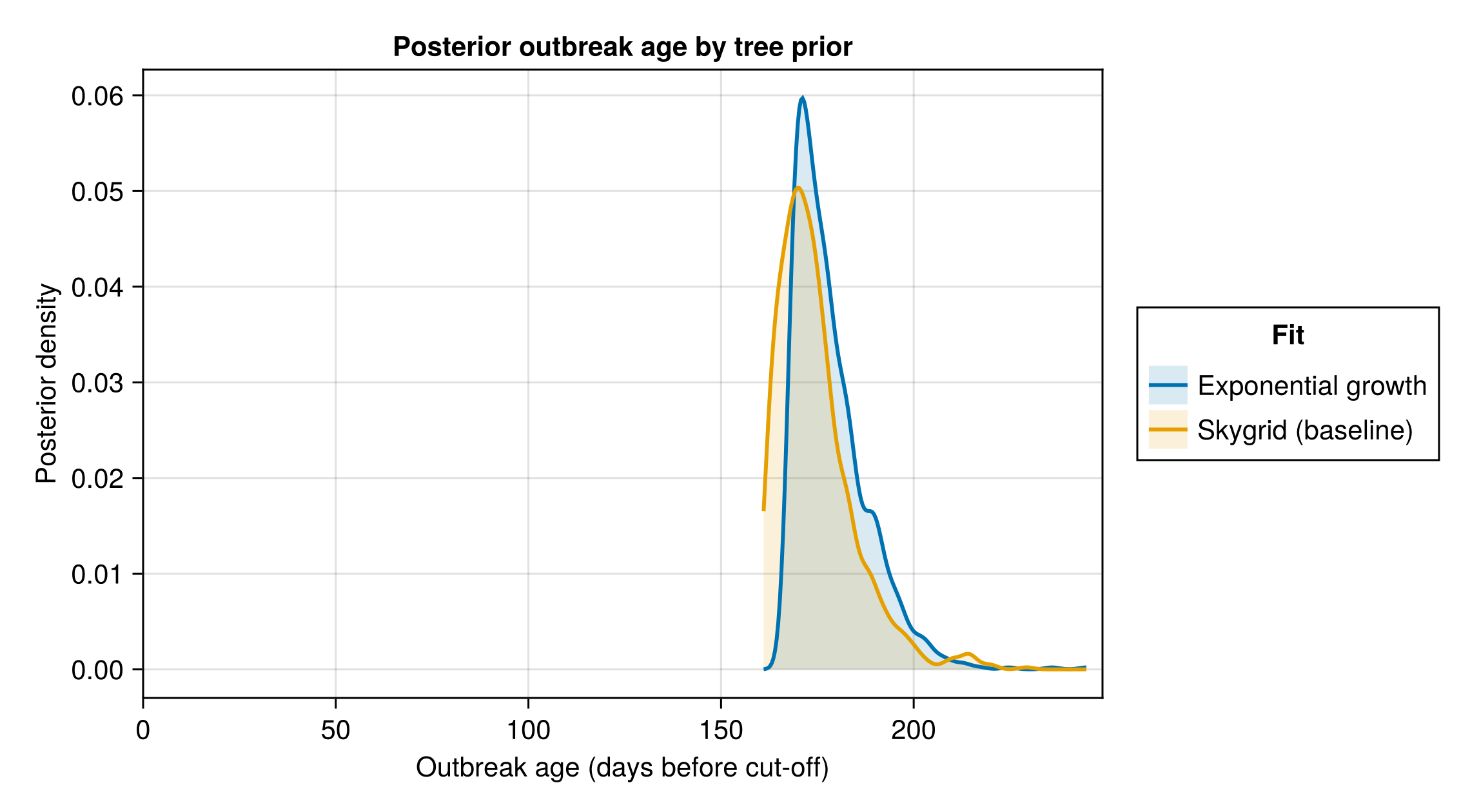
Saving sensitivity results
The stream-comparison and frozen-fit tables and the per-stream reproduction number figure are written to the shared output directory. The main analysis writes the rest, so the combined release and summary dashboard pick up both pages' outputs.
Write sensitivity outputs
output_dir = get(ENV, "BVD_OUTPUT_DIR",
    joinpath(pkgdir(BVDOutbreakSize), "output"))
mkpath(output_dir)
CSV.write(joinpath(output_dir, "cumulative_cases_by_stream.csv"),
    streams_C_table)
CSV.write(joinpath(output_dir, "frozen_matched_cutoffs.csv"),
    frozen_streams_table)

# The one-week-back validation forecast, in the same archive format as the
# release forecast, so the frozen "last week versus now" forecast is recorded
# as a release asset alongside the forecast it is scored against.
CSV.write(joinpath(output_dir, "forecast_validation.csv"),
    forecast_archive([(7, validation_forecast)];
        made_date = frozen_lastweek.o.cutoff, thin = 5))

# The per-stream reproduction-number figure for the summary dashboard; the
# main analysis writes the other three dashboard figures.
dashboard_dir = joinpath(
    pkgdir(BVDOutbreakSize), "docs", "src", "summary_assets")
mkpath(dashboard_dir)
CairoMakie.save(joinpath(dashboard_dir, "rt_streams.png"), stream_rt_fig)