Analysis walkthrough

The Epuyén 2018–19 outbreak in north-west Patagonia was the first cluster where person-to-person Andes hantavirus transmission was documented at scale. The line list bundled with this package is hand-encoded from Table S2 of Martínez et al. 2020 — 34 cases with exposure windows, symptom-onset dates, and attributed source cases.

This page fits the joint model in TransmissionLinelist.jl to that line list and renders the headline outputs. Four quantities are estimated together: the incubation period, the transmission timing of each secondary relative to its source's symptom onset (δ), a weekly time-varying reproduction number R(t), and the offspring dispersion k of a Negative-Binomial. Exposure and onset dates are interval-censored. The model handles that by giving each case a continuous latent infection time and a continuous latent onset time, each sampled within its recorded window. Generation interval and serial interval are derived in post-processing as the transmission timing plus an incubation period (the source's for GI, the secondary's for SI). Fitting all four jointly propagates uncertainty between them that a delay-then-R(t) pipeline would lose.

Priors, the data-augmentation construction, and per-pair GI > 0 constraint are detailed on the Model page. Caveats around exposure encoding, late R(t) bins, and right-truncation are on the Limitations page.

using TransmissionLinelist
using Chain
using DataFrames
using DataFramesMeta
using Distributions: LogNormal
using FlexiChains
using Printf
using Random
using Statistics: quantile
using CairoMakie
using AlgebraOfGraphics
using PairPlots

Random.seed!(20260508)

Random.TaskLocalRNG()

Load the line list

load_linelist parses the bundled CSV and drops the _alt sensitivity rows. build_data re-encodes exposure / onset windows as day offsets from t0 (60 days before the first onset), and prepare_rt_edges builds the weekly R(t) knot dates from the same origin. Passing those into joint_model instantiates the Turing model directly.

ll = load_linelist()
d = build_data(ll)
edges = prepare_rt_edges(d.t0)
model = joint_model(d, edges)

@chain ll begin
    @select(:patient_id, :exposure_lower, :exposure_upper,
        :onset_date, :source_case, :Z)
    first(8)
end

8×6 DataFrame

Row	patient_id	exposure_lower	exposure_upper	onset_date	source_case	Z
	String	Date?	Date?	Date	String15?	Int64
1	1	missing	missing	2018-11-03	missing	5
2	2	2018-11-03	2018-11-03	2018-11-23	1	6
3	3	2018-11-03	2018-11-03	2018-11-20	1	0
4	4	2018-11-03	2018-11-03	2018-11-27	1	0
5	5	2018-11-03	2018-11-03	2018-11-26	1	1
6	6	2018-11-03	2018-11-03	2018-11-25	1	0
7	7	2018-11-23	2018-11-23	2018-12-07	2	0
8	8	2018-11-23	2018-11-23	2018-12-13	2	1

What the data looks like

plot_data(ll)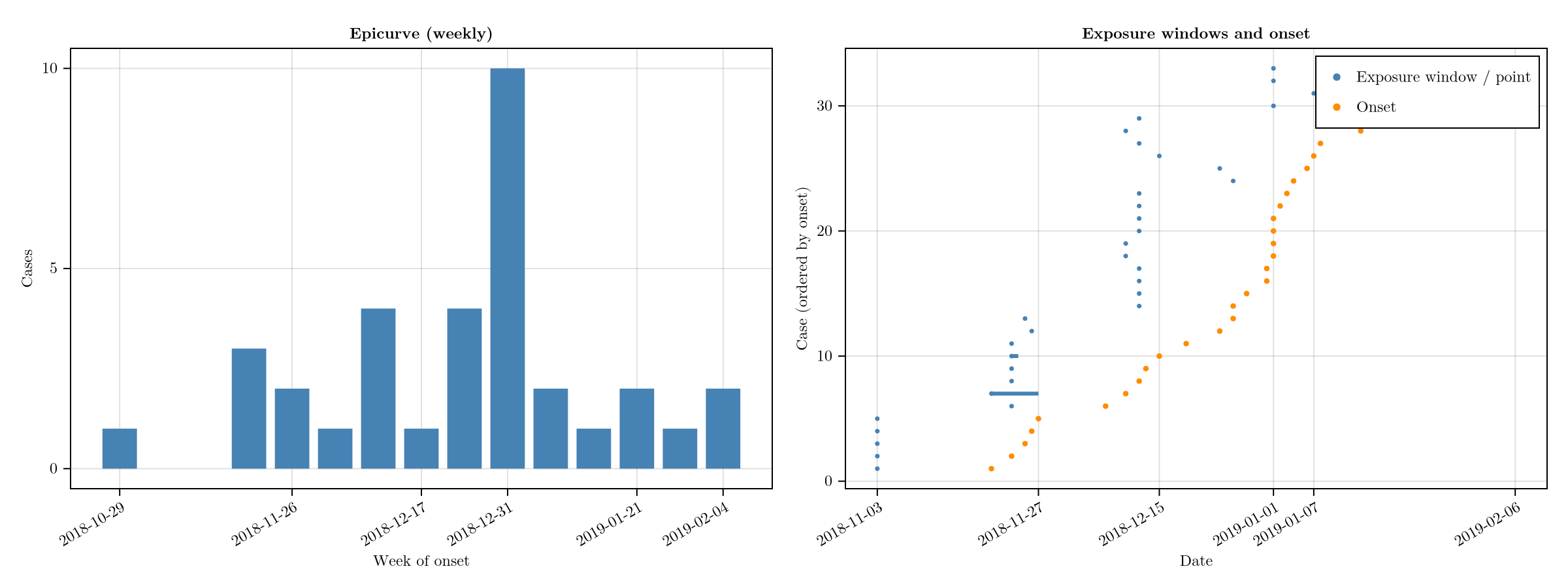

Model

@model function joint_model(d, edges;
        incubation = incubation_model(),
        transmission = transmission_delta_model(),
        rt = random_walk_rt_model(length(edges)),
        dispersion = nb_dispersion_model(),
        cases = case_model)
    delays ~ to_submodel(
        delays_only_model(d; incubation, transmission), false)
    case_obs ~ to_submodel(
        cases(d.Zobs, edges, delays.T_onset, delays.p;
            rt, dispersion), false)
end

Prior predictives

Implied prior distributions for the incubation period, transmission timing δ, and the derived generation / serial interval before any data are seen.

plot_prior_predictives()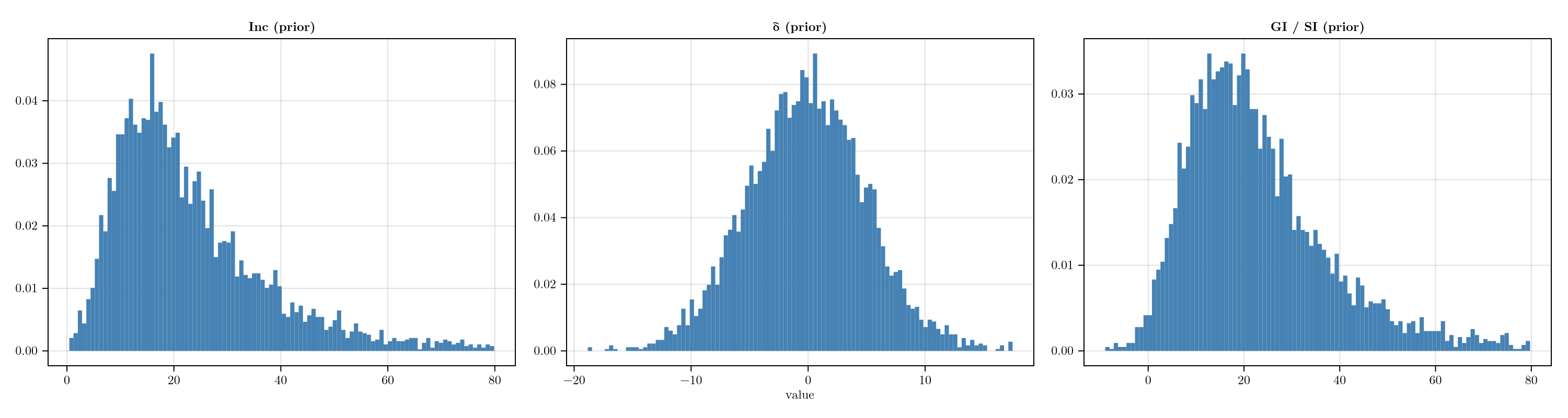

Fitting

sample_fit wraps the package's default NUTS configuration: Mooncake reverse-mode AD, chains initialised from the prior, 1000 post-warmup draws across 4 chains, target_accept = 0.95.

chn = sample_fit(model)

╭─FlexiChain (1000 iterations, 4 chains) ──────────────────────────────────────╮
│ ↓ iter  = 501:1500                                                           │
│ → chain = 1:4                                                                │
│                                                                              │
│ Parameters (12) ── AbstractPPL.VarName                                       │
│  Float64          μ_inc, σ_inc, μ_δ, σ_δ, σ_rw, log_R_init, phi_inv_sqrt, k  │
│  Vector{Float64}  T_onset, T_inf, ε, log_R                                   │
│                                                                              │
│ Extras (14)                                                                  │
│  Int64    n_steps, tree_depth                                                │
│  Bool     is_accept, numerical_error                                         │
│  Float64  acceptance_rate, log_density, hamiltonian_energy,                  │
│           hamiltonian_energy_error, max_hamiltonian_energy_error, step_size, │
│           nom_step_size, logprior, loglikelihood, logjoint                   │
╰──────────────────────────────────────────────────────────────────────────────╯

Drop a compact regression snapshot to output/regression/analysis.csv for the docs CI to diff against the checked-in baseline. Flags any future PR whose fit drifts outside MCMC noise.

save_regression_summary(
    joinpath(@__DIR__, "..", "..", "output",
        "regression", "analysis.csv"), chn)

"/home/runner/work/andv-linelist-analysis/andv-linelist-analysis/docs/build/../../output/regression/analysis.csv"

Diagnostics

Maximum R̂, minimum bulk ESS, divergence count, and wall-clock sampling time (seconds, approximated by the slowest chain under MCMCThreads).

diagnostics_table(chn)

1×4 DataFrame

Row	rhat_max	ess_min	divergences	runtime_seconds
	Float64	Float64	Int64	Float64
1	1.00697	2328.28	0	137.194

Key outputs

summary_table(chn)

8×4 DataFrame

Row	quantity	median	lower_95	upper_95
	String	Float64	Float64	Float64
1	Incubation mean (d)	22.5527	20.2351	25.5767
2	Incubation 95th pct (d)	36.2087	31.1677	44.4239
3	Incubation 99th pct (d)	45.0269	37.3469	58.3775
4	μ_δ (d from source onset)	0.172518	-0.170569	0.495142
5	σ_δ (d)	0.609041	0.456188	0.835941
6	GI / SI mean (d)	22.714	20.3861	25.6692
7	GI / SI SD (d)	7.38946	5.57285	10.4537
8	NB dispersion k	0.303329	0.133212	0.876006

Observed offspring counts

Each case is plotted at its observed offspring count Z (with small vertical jitter to break ties) against time. Thin segments are posterior draws of the latent infection time T_inf joined to the latent onset time T_onset; filled dots are the posterior medians of T_inf and hollow dots the medians of T_onset. Index and sourced cases are coloured separately. This is a direct view of what the model has to explain before R(t) enters the picture; the posterior-predictive comparison against modelled offspring counts comes later under plot_z_ppc.

plot_z_dumbbell(chn, d)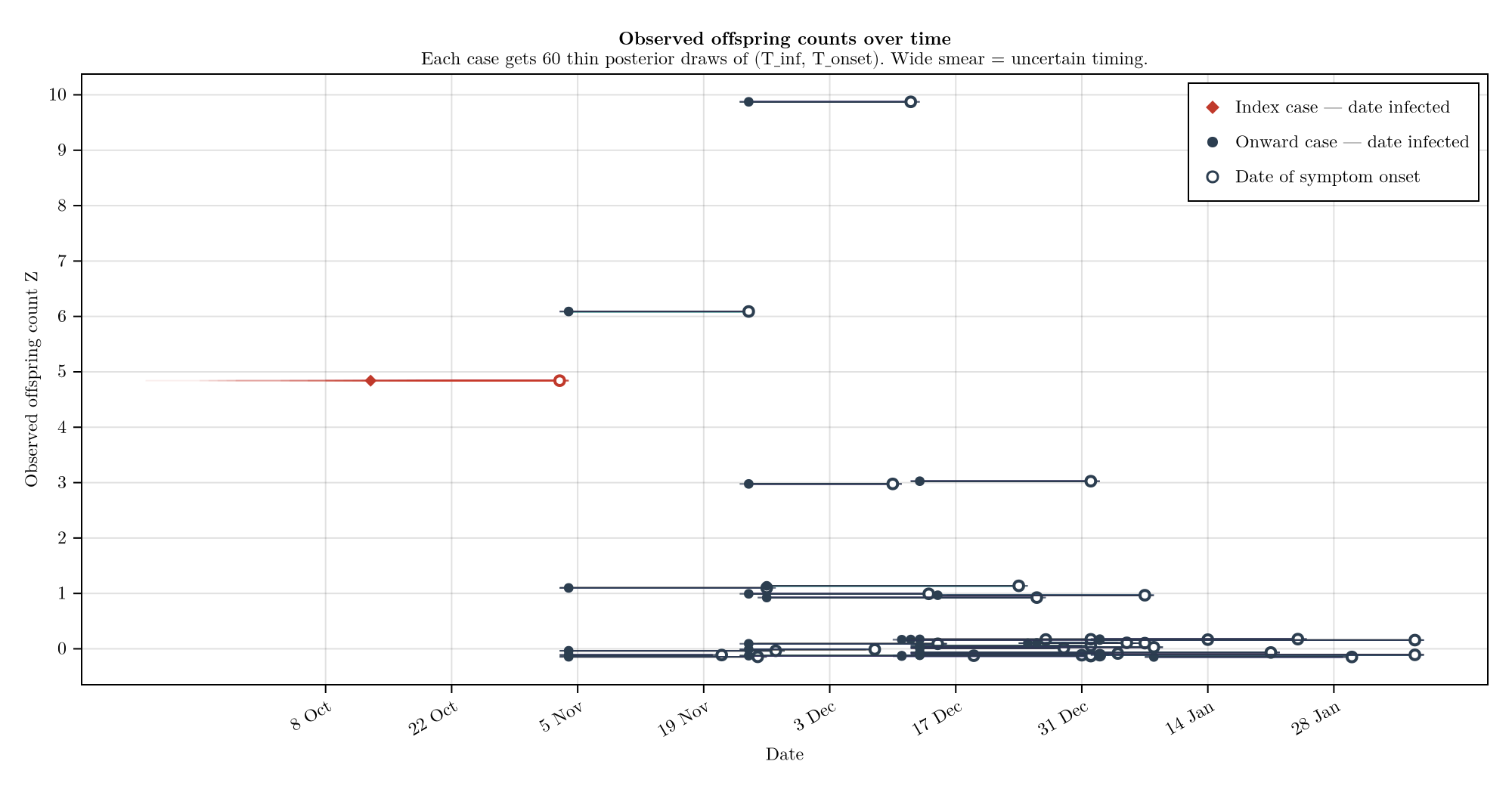

R(t) over weekly knots

Spaghetti of thinned posterior draws through the weekly knots (linearly interpolated); reverts to the prior in late-January knots where cases are thin (see Limitations).

plot_rt(chn)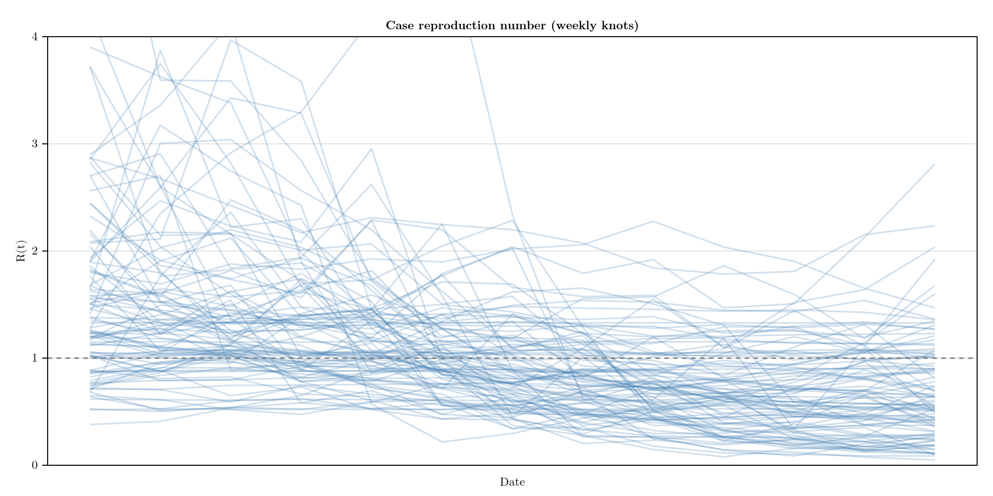

Pair plot of population parameters

Corner plot for μ_inc, σ_inc, μ_δ, σ_δ, k.

plot_pair(chn)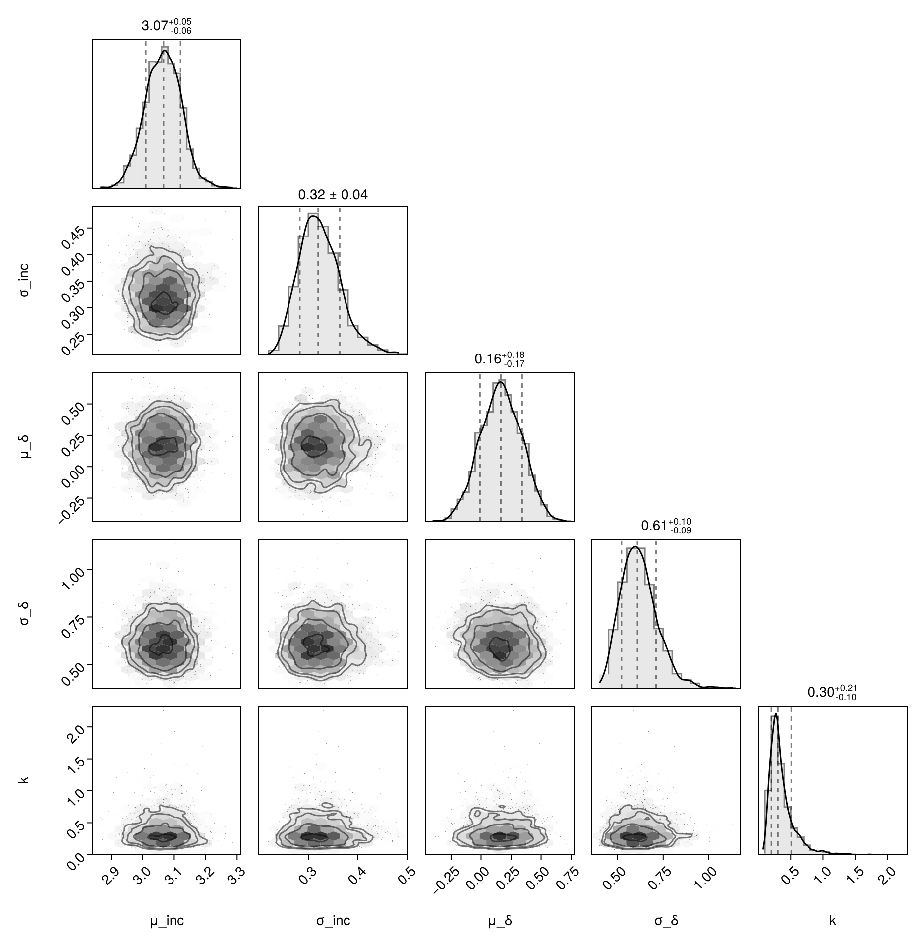

Predictive distributions for the delays

Implied population distributions for the incubation period, transmission timing δ, and the derived generation and serial intervals under the fitted posterior — i.e. what a new case or transmission pair would look like. This is not a check against the observed data; for that see the sense-check and PPC panels below. Inc and δ panels show the posterior over the parametric density (median PDF with a 95% pointwise ribbon across draws) overlaid with one predictive realisation per draw; GI and SI show the predictive-sample histogram only.

plot_predictive_distributions(chn)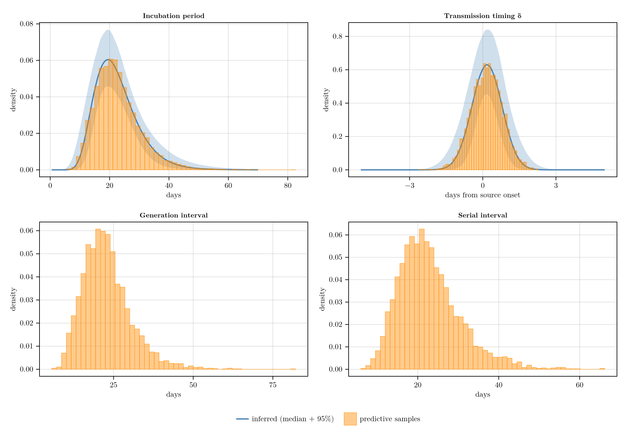

δ sense check

Compare the per-pair posterior medians of δ to the fitted population Normal(μ_δ, σ_δ).

plot_delta_sense_check(chn, d)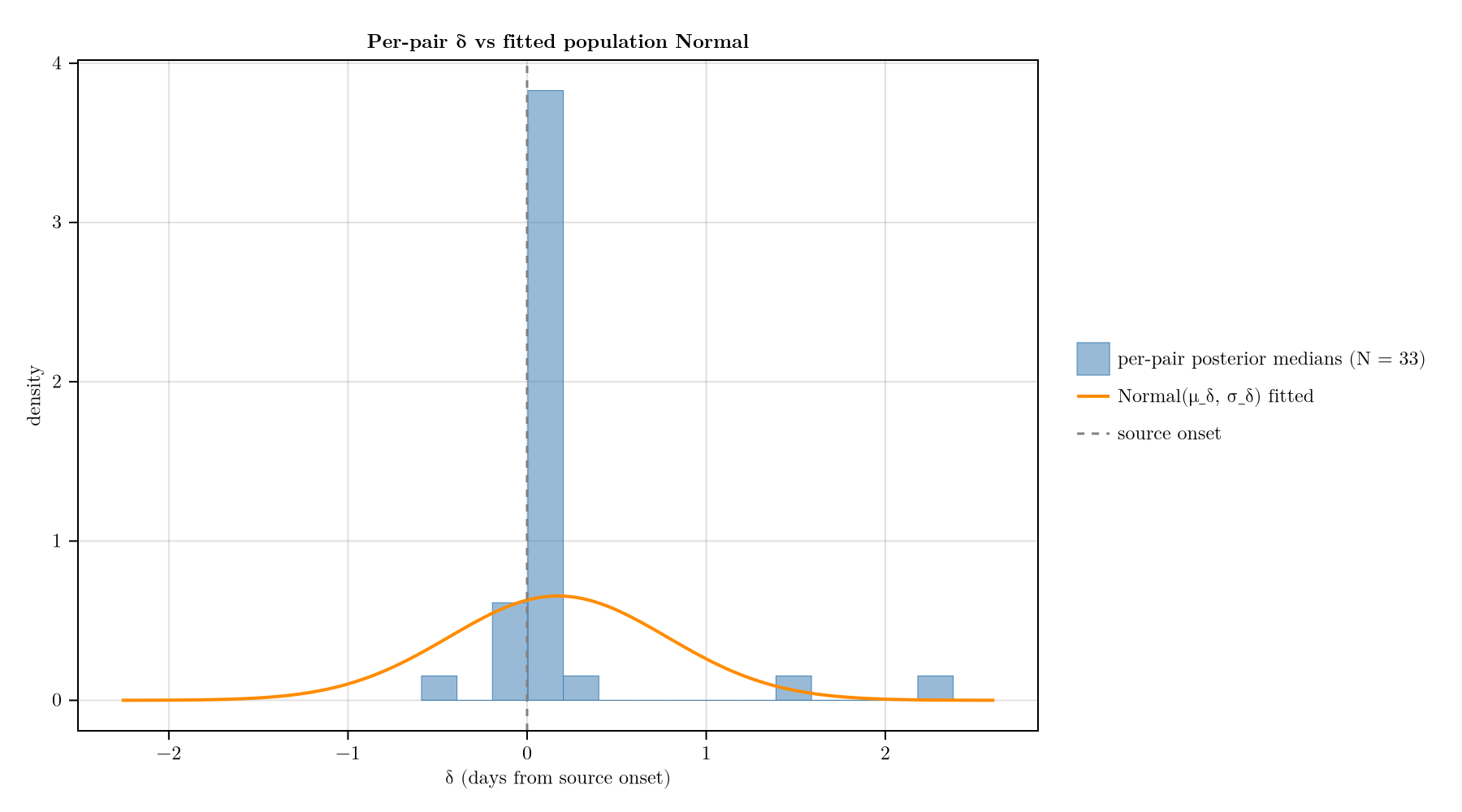

Incubation-period sense check

Compare the per-case posterior medians of T_onset[i] − T_inf[i] to the fitted population LogNormal(μ_inc, σ_inc).

plot_inc_sense_check(chn, d)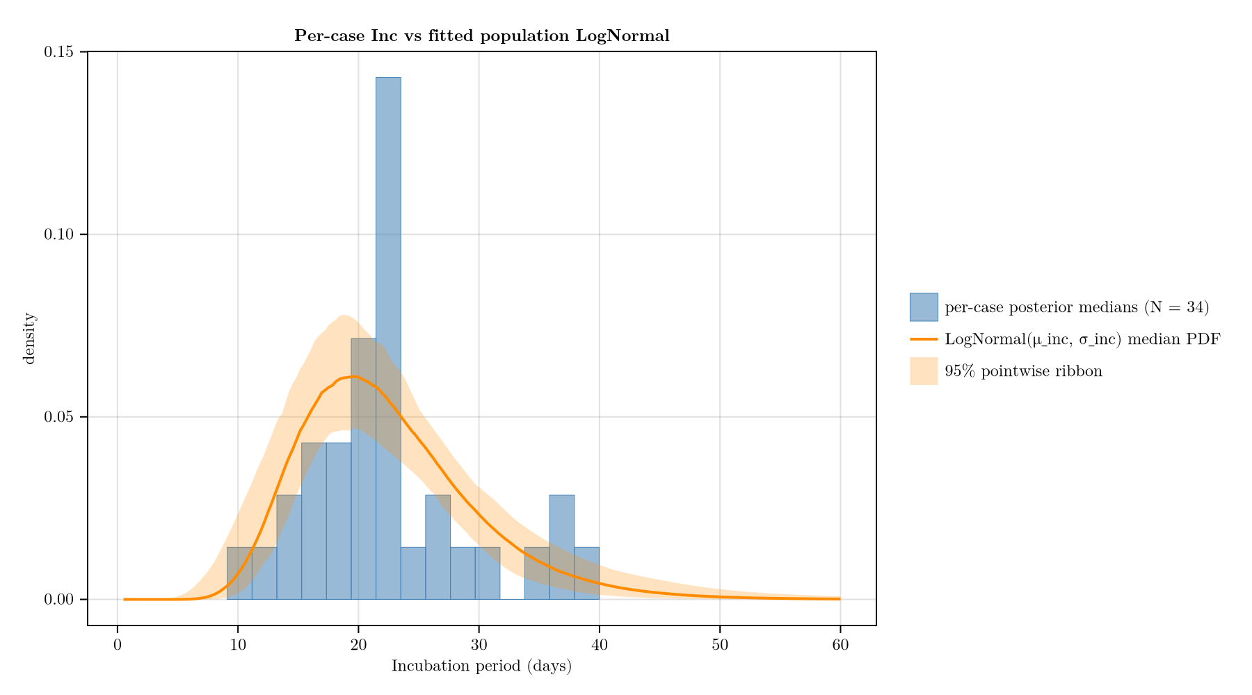

Offspring posterior-predictive check

Joint-draw posterior-predictive check. For each posterior draw, replicate Z_rep[i] ~ NegativeBinomial(k, k/(k+R_i)) per case, with R_i = exp(log_R_at(T_inf[i], edges, log_R)) evaluated at the same draw's T_inf[i], log_R, and k (matching the model's likelihood, clamp and all). The left panel compares frequencies of each Z value against the observed line list. The right column has three stacked subpanels — one per discrete test statistic (sum(Z), max(Z), count(Z = 0)) — each showing the histogram of the replicated statistic with the observed value as a dashed vertical rule.

plot_z_ppc(model, chn, d; edges = edges)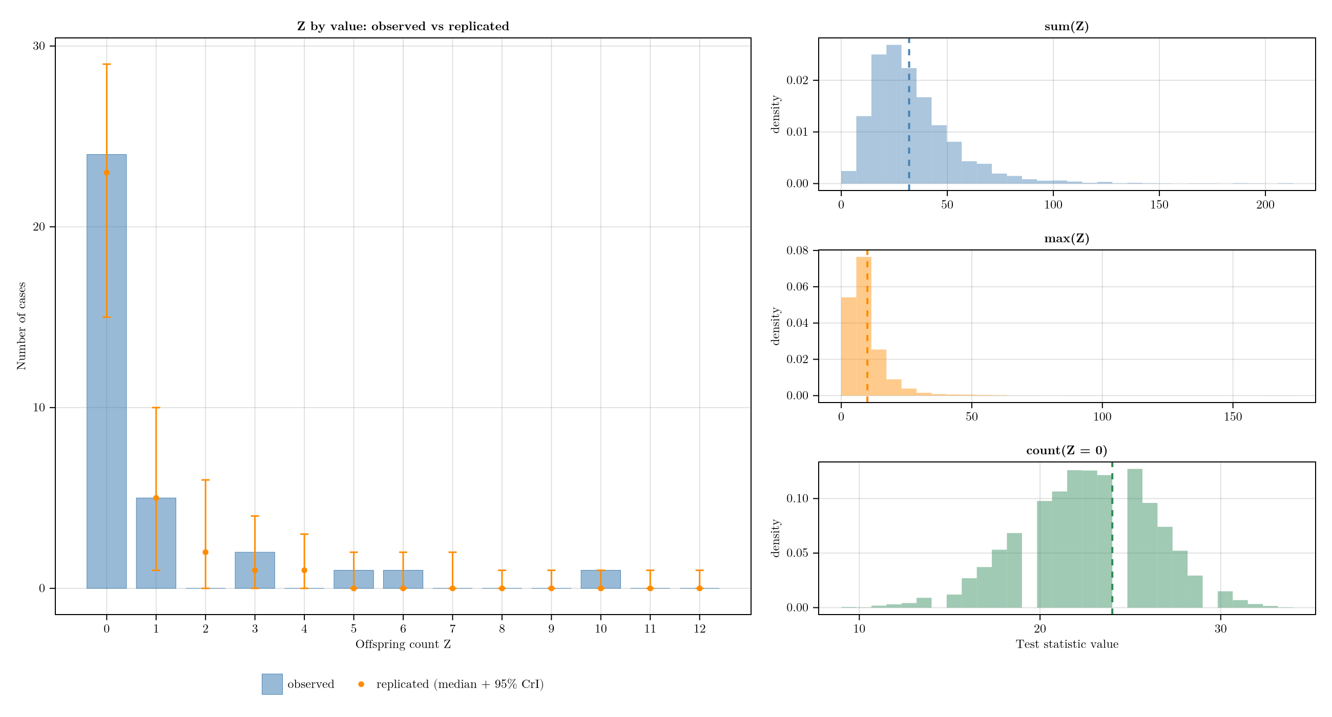

Numeric values for each test statistic — observed, replicated median + 95% CrI, and the two-sided Bayesian posterior-predictive p-value 2 · min(P(T_rep ≥ T_obs), P(T_rep ≤ T_obs)).

z_ppc_summary(model, chn, d; edges = edges)

3×6 DataFrame

Row	statistic	observed	rep_median	rep_lower_95	rep_upper_95	p_ppp
	String	Float64	Float64	Float64	Float64	Float64
1	sum(Z)	32.0	30.0	9.0	85.0	0.92
2	max(Z)	10.0	8.0	2.0	29.0	0.708
3	count(Z = 0)	24.0	23.0	15.0	29.0	0.873

Comparison with Martínez et al. 2020

The line list used here is hand-encoded from Table S2 of Martínez et al. 2020, so the joint model and the source paper are fitted to the same outbreak. The table below places our posterior estimates next to the values that the NEJM paper reports for the same outbreak, with our column built directly from the fitted chain in scope (chn). Martínez values are pasted from the abstract and main text of the paper; where the paper does not report a quantity we estimate, the study columns are left as missing rather than fabricated. Our our_80_ci column is the central 80% credible interval (10th–90th percentile across posterior draws), chosen as a band that is comparable in tail mass to the empirical 9–40 day incubation range reported by the paper.

post = summarise(chn)

inc_median = exp.(post.μ_inc)
inc_q95 = [quantile(LogNormal(post.μ_inc[i], post.σ_inc[i]), 0.95)
           for i in eachindex(post.μ_inc)]
rt_peak = [maximum(exp(post.log_R_chain[b][i])
           for b in eachindex(post.log_R_chain))
           for i in eachindex(post.μ_inc)]

q10(x) = quantile(x, 0.1)
q50(x) = quantile(x, 0.5)
q90(x) = quantile(x, 0.9)
fmt2(x) = @sprintf("%.2f", x)
ci80(x) = string(fmt2(q10(x)), "–", fmt2(q90(x)))

martinez_rows = [
    (parameter = "Incubation period — median (d)",
        study_value = "21",
        study_ci = "range 9–40",
        our_median = fmt2(q50(inc_median)),
        our_80_ci = ci80(inc_median),
        notes = "Martínez reports the empirical median and range of " *
                "observed incubation periods; our value is the median " *
                "of the fitted LogNormal."),
    (parameter = "Incubation period — μ_inc (log-scale mean)",
        study_value = "missing",
        study_ci = "missing",
        our_median = fmt2(q50(post.μ_inc)),
        our_80_ci = ci80(post.μ_inc),
        notes = "Martínez does not fit a parametric incubation " *
                "distribution, so no log-scale mean is reported."),
    (parameter = "Incubation period — σ_inc (log-scale SD)",
        study_value = "missing",
        study_ci = "missing",
        our_median = fmt2(q50(post.σ_inc)),
        our_80_ci = ci80(post.σ_inc),
        notes = "Not reported by Martínez (no parametric " *
                "distribution fitted)."),
    (parameter = "Incubation period — 95th percentile (d)",
        study_value = "missing",
        study_ci = "missing",
        our_median = fmt2(q50(inc_q95)),
        our_80_ci = ci80(inc_q95),
        notes = "Martínez reports the maximum observed value (40 d) " *
                "rather than a fitted 95th percentile."),
    (parameter = "Serial interval — mean (d)",
        study_value = "missing",
        study_ci = "missing",
        our_median = fmt2(q50(post.mean_gi_si)),
        our_80_ci = ci80(post.mean_gi_si),
        notes = "Martínez does not report a serial-interval " *
                "distribution; our SI mean and SD are derived from " *
                "the joint posterior over δ and the incubation period."),
    (parameter = "Serial interval — SD (d)",
        study_value = "missing",
        study_ci = "missing",
        our_median = fmt2(q50(post.sd_gi_si)),
        our_80_ci = ci80(post.sd_gi_si),
        notes = "As above; GI and SI share the same marginal in this " *
                "model so the same row covers the generation interval."),
    (parameter = "Generation interval — mean (d)",
        study_value = "missing",
        study_ci = "missing",
        our_median = fmt2(q50(post.mean_gi_si)),
        our_80_ci = ci80(post.mean_gi_si),
        notes = "Martínez does not report a generation-interval " *
                "distribution."),
    (parameter = "Offspring dispersion k",
        study_value = "missing",
        study_ci = "missing",
        our_median = fmt2(q50(post.k)),
        our_80_ci = ci80(post.k),
        notes = "Martínez identifies three super-spreaders " *
                "qualitatively but does not fit a Negative-Binomial " *
                "dispersion."),
    (parameter = "Maximum R(t) over weekly knots",
        study_value = "2.12",
        study_ci = "missing",
        our_median = fmt2(q50(rt_peak)),
        our_80_ci = ci80(rt_peak),
        notes = "Martínez reports a pre-intervention R of 2.12 " *
                "(falling to 0.96 after isolation); no CI given. " *
                "Our value is the per-draw maximum of exp(log_R) " *
                "across weekly knots, so it sits above any single " *
                "weekly posterior median."),
    (parameter = "Secondary attack rate",
        study_value = "missing",
        study_ci = "missing",
        our_median = "missing",
        our_80_ci = "missing",
        notes = "Martínez describes super-spreading qualitatively " *
                "without a numeric SAR; our model targets R(t) and " *
                "k rather than a per-contact attack rate, so neither " *
                "side reports a comparable value.")
]

DataFrame(martinez_rows)

10×6 DataFrame

Row	parameter	study_value	study_ci	our_median	our_80_ci	notes
	String	String	String	String	String	String
1	Incubation period — median (d)	21	range 9–40	21.42	19.93–23.02	Martínez reports the empirical median and range of observed incubation periods; our value is the median of the fitted LogNormal.
2	Incubation period — μ_inc (log-scale mean)	missing	missing	3.06	2.99–3.14	Martínez does not fit a parametric incubation distribution, so no log-scale mean is reported.
3	Incubation period — σ_inc (log-scale SD)	missing	missing	0.32	0.27–0.38	Not reported by Martínez (no parametric distribution fitted).
4	Incubation period — 95th percentile (d)	missing	missing	36.21	32.75–40.93	Martínez reports the maximum observed value (40 d) rather than a fitted 95th percentile.
5	Serial interval — mean (d)	missing	missing	22.71	21.16–24.47	Martínez does not report a serial-interval distribution; our SI mean and SD are derived from the joint posterior over δ and the incubation period.
6	Serial interval — SD (d)	missing	missing	7.39	6.16–9.18	As above; GI and SI share the same marginal in this model so the same row covers the generation interval.
7	Generation interval — mean (d)	missing	missing	22.71	21.16–24.47	Martínez does not report a generation-interval distribution.
8	Offspring dispersion k	missing	missing	0.30	0.18–0.59	Martínez identifies three super-spreaders qualitatively but does not fit a Negative-Binomial dispersion.
9	Maximum R(t) over weekly knots	2.12	missing	1.62	0.91–3.24	Martínez reports a pre-intervention R of 2.12 (falling to 0.96 after isolation); no CI given. Our value is the per-draw maximum of exp(log_R) across weekly knots, so it sits above any single weekly posterior median.
10	Secondary attack rate	missing	missing	missing	missing	Martínez describes super-spreading qualitatively without a numeric SAR; our model targets R(t) and k rather than a per-contact attack rate, so neither side reports a comparable value.