Why stratify, and why pool
The CFR often varies by group – age, treatment centre, calendar period – and a per-group estimate is frequently required. Two limiting cases bracket the options. Fitting each group independently (no pooling) gives high-variance estimates where a group’s sample is small. Fitting one CFR for all groups (complete pooling) ignores between-group variation.
Partial pooling lies between the two: each group’s CFR is
drawn from a common distribution, so groups with more data are estimated
close to independently while groups with less data are shrunk toward the
shared mean. cfrnow is an epidist model, so
prob takes a brms formula and pooling is a
one-line change: prob ~ (1 | group).
A six-site line list
We simulate six treatment centres: two large (n = 450, 250) and four small (n = 15–20), with true CFRs spread around a common mean. The large sites pin the shared mean; the small ones carry little information on their own, so shrinkage acts mainly on them. Site labels are synthetic.
library(cfrnow)
#> Loading required package: distspec
#>
#> Attaching package: 'distspec'
#> The following objects are masked from 'package:stats':
#>
#>     Gamma, sd
set.seed(20260714)

sites <- data.frame(
  site = c("A", "B", "C", "D", "E", "F"),
  n    = c(450, 250, 20, 15, 15, 18),
  cfr  = c(0.45, 0.50, 0.30, 0.65, 0.35, 0.60)
)

death_delay    <- LogNormal(mean = 11, sd = 6.5)
recovery_delay <- LogNormal(mean = 16, sd = 8)

ll <- do.call(rbind, Map(function(s, n, cfr) {
  cbind(
    simulate_linelist(
      n = n, cfr = cfr, delay = death_delay,
      recovery = recovery_delay, onset_days = 45
    ),
    site = s
  )
}, sites$site, sites$n, sites$cfr))

d <- prepare_cfr_data(ll, obs_time = as.Date("2026-02-20"), covariates = "site")
c(cases = d$n_cases, deaths = d$n_deaths)
#>  cases deaths
#>    768    331
Three fits: complete, no, and partial pooling
The only thing that changes across the three fits is the CFR formula; the delay and recovery delay are co-estimated in each. (Two short chains keep the build time short; use more for inference.)
otd <- LogNormal(meanlog = Normal(2.4, 0.2), sdlog = Normal(0.5, 0.15))
otr <- LogNormal(meanlog = Normal(2.7, 0.2), sdlog = Normal(0.5, 0.15))
args <- list(
  delay = otd, recovery_delay = otr, prob_prior = Beta(1, 1),
  backend = "cmdstanr", chains = 2, iter = 1000, refresh = 0, seed = 1
)

# complete pooling: a single CFR
fit_pool    <- do.call(fit_cfr, c(list(d, formula = brms::bf(mu ~ 1, prob ~ 1)), args))

# no pooling: an independent CFR per site (one estimated logit-CFR per site)
fit_sep     <- do.call(fit_cfr, c(list(d, formula = brms::bf(mu ~ 1, prob ~ 0 + site)), args))

# partial pooling: per-site CFR shrunk to a common mean
fit_partial <- do.call(fit_cfr, c(list(d, formula = brms::bf(mu ~ 1, prob ~ (1 | site))), args))
Reading the estimates
For the complete-pool fit, summary() reports a single
prob row:
summary(fit_pool)
#>        quantity       mean       q2.5        q50      q97.5      rhat ess_bulk
#> 1          prob  0.5071483  0.4661708  0.5074665  0.5478851 0.9999676 889.8351
#> 2    delay_mean 11.8390416 10.7503330 11.8292516 13.1068921 1.0034747 686.6163
#> 3      delay_sd  8.2789703  6.8811035  8.2137501  9.9473744 1.0030746 731.2997
#> 4 recovery_mean 15.3699938 14.3700185 15.3715181 16.4850453 1.0118875 681.2057
#> 5   recovery_sd  7.7295416  6.6419162  7.6999960  8.9705999 1.0103824 586.4672
For a grouped fit it reports one prob[<site>] row
per site:
summary(fit_sep)
#>         quantity       mean       q2.5        q50      q97.5     rhat ess_bulk
#> 1        prob[A]  0.4785987  0.4291501  0.4787721  0.5302094 1.004340 1332.544
#> 2        prob[B]  0.5635791  0.4935825  0.5636292  0.6326111 1.002791 1619.235
#> 3        prob[C]  0.1906897  0.0607537  0.1800252  0.3751848 1.002084 2187.687
#> 4        prob[D]  0.5222949  0.2663020  0.5227338  0.7681408 1.003810 1782.922
#> 5        prob[E]  0.5950808  0.3144592  0.5947216  0.8460654 1.000549 2020.341
#> 6        prob[F]  0.7729615  0.5448519  0.7867617  0.9460552 1.000770 1723.954
#> 7     delay_mean 11.8646173 10.8377074 11.8383652 12.9919330 1.001511 1367.777
#> 8       delay_sd  8.3103476  6.9195949  8.2771800  9.9138624 1.003348 1381.695
#> 9  recovery_mean 15.3760850 14.4455879 15.3750048 16.4039886 1.000365 1387.057
#> 10   recovery_sd  7.7379201  6.6077130  7.7004354  9.0237652 1.001666 1329.814
Collect those per-site CFR rows from the two grouped fits for the figure below; the complete-pool fit supplies the shared mean.
cfr_rows <- function(fit, approach) {
  s <- summary(fit)
  r <- s[grepl("^prob\\[", s$quantity), ] # the prob[<site>] rows
  data.frame(
    approach = approach,
    site = sub("^prob\\[(.*)\\]$", "\\1", r$quantity),
    median = r$q50, lower = r$q2.5, upper = r$q97.5
  )
}

est <- rbind(cfr_rows(fit_sep, "no pool"), cfr_rows(fit_partial, "partial pool"))
est <- merge(est, sites[, c("site", "n", "cfr")], by = "site")
names(est)[names(est) == "cfr"] <- "truth"

s_pool <- summary(fit_pool)
pool_mean <- s_pool$q50[s_pool$quantity == "prob"]
Shrinkage
Each site shows its no-pool and partial-pool estimate against the truth (×) and the complete-pool mean (dotted). For the large sites (A, B) the two estimates nearly coincide. For the small sites (C–F) the no-pool interval is wide and the estimate noisy; partial pooling pulls it toward the mean and narrows the interval sharply – lower variance at the cost of some bias.
library(ggplot2)
est$approach <- factor(est$approach, levels = c("no pool", "partial pool"))
est$site <- factor(est$site, levels = rev(sites$site))

ggplot(est, aes(median, site, colour = approach)) +
  geom_vline(xintercept = pool_mean, linetype = 3) +
  geom_point(aes(x = truth), shape = 4, size = 2.4, colour = "grey30") +
  geom_pointrange(aes(xmin = lower, xmax = upper), position = position_dodge(width = 0.55)) +
  scale_y_discrete(labels = function(s) paste0(s, "  (n=", sites$n[match(s, sites$site)], ")")) +
  labs(
    x = "CFR: median & 95% CrI   (× = truth, dotted = complete-pool mean)",
    y = NULL, colour = NULL
  ) +
  theme_minimal()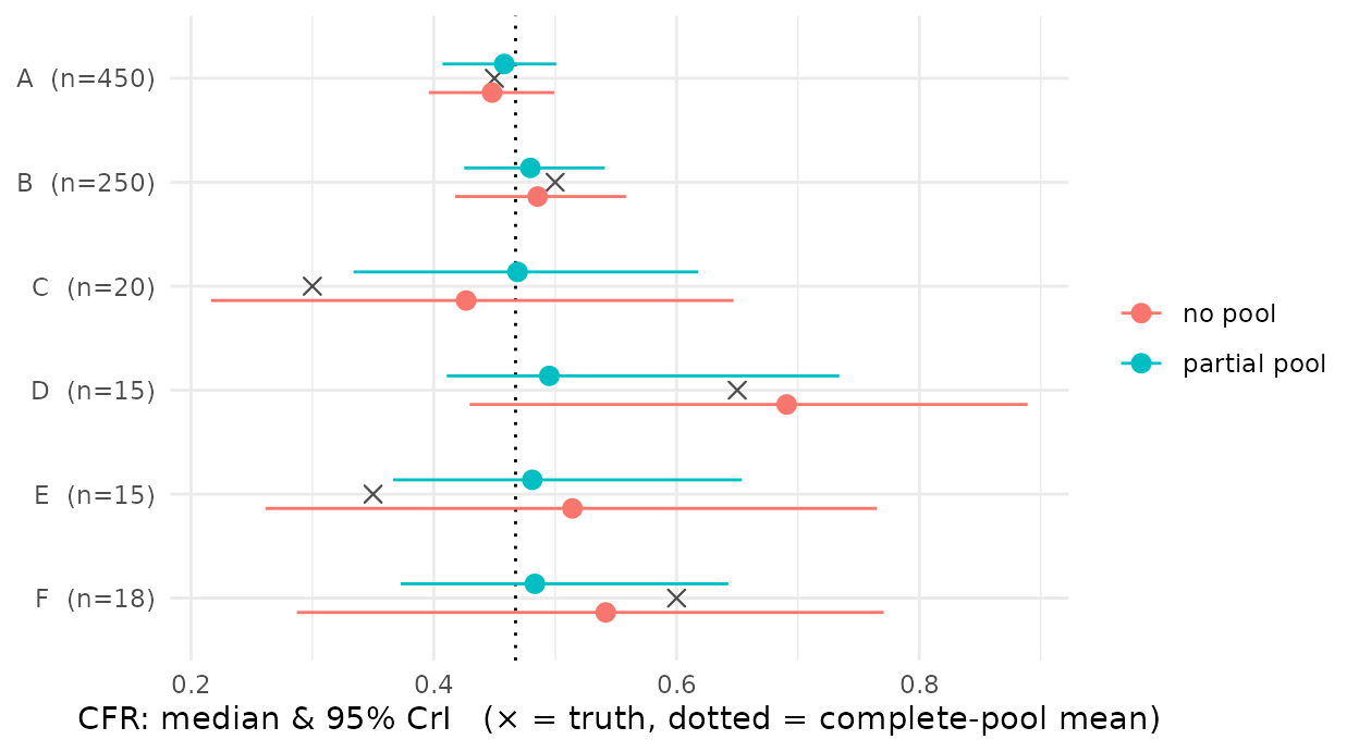
Varying the delay by group
A pooled onset-to-death delay that appears irregular is often a mixture of several populations. If sites resolve on different timescales, pool the delay by site as well, so each retains its own onset-to-death distribution rather than contributing to a single multimodal one:
Check the fit
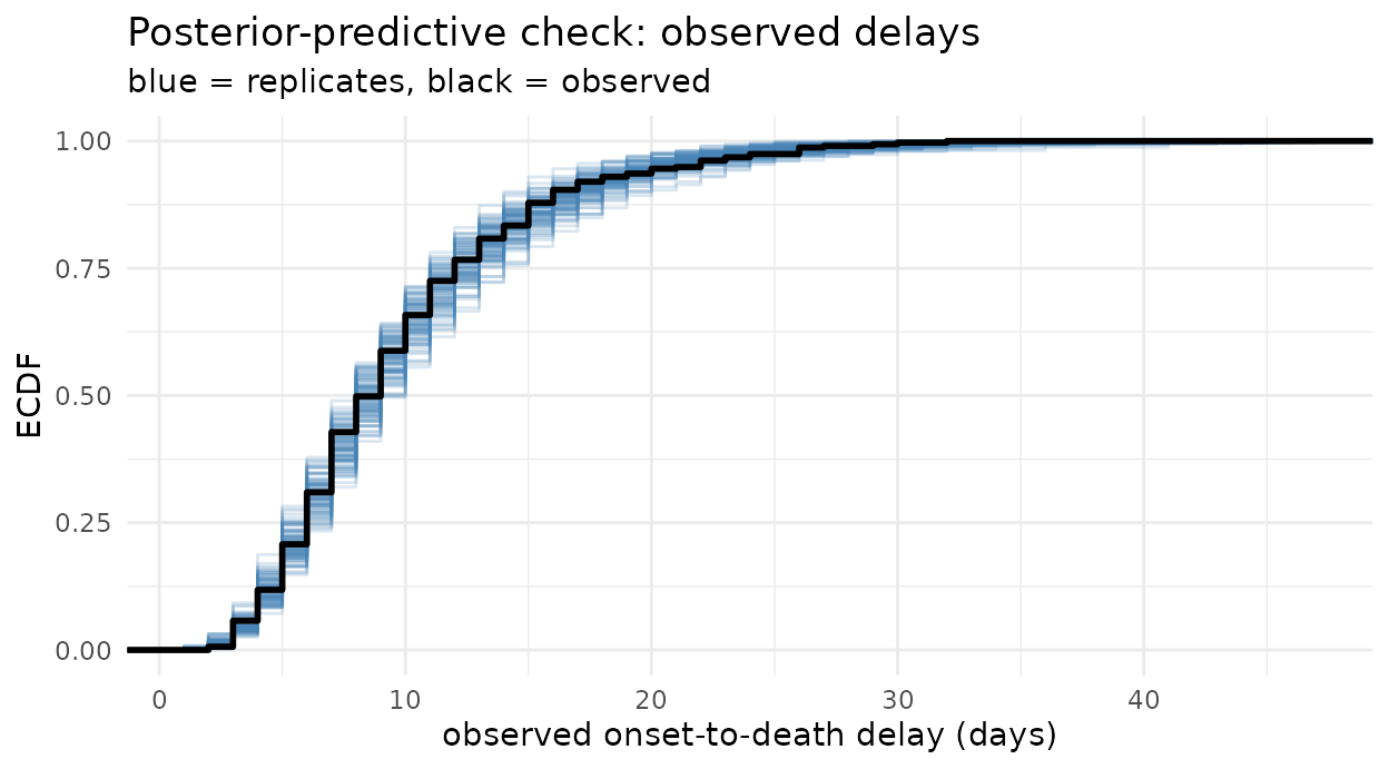
Check that the parametric delay reproduces the observed delays; the real-time correction depends on extrapolating that delay’s tail.
pp_check_cfr(fit_partial, type = "delay")