Determines bias from predictive Monte-Carlo samples. The function automatically recognises whether forecasts are continuous or integer valued and adapts the Bias function accordingly.
Value
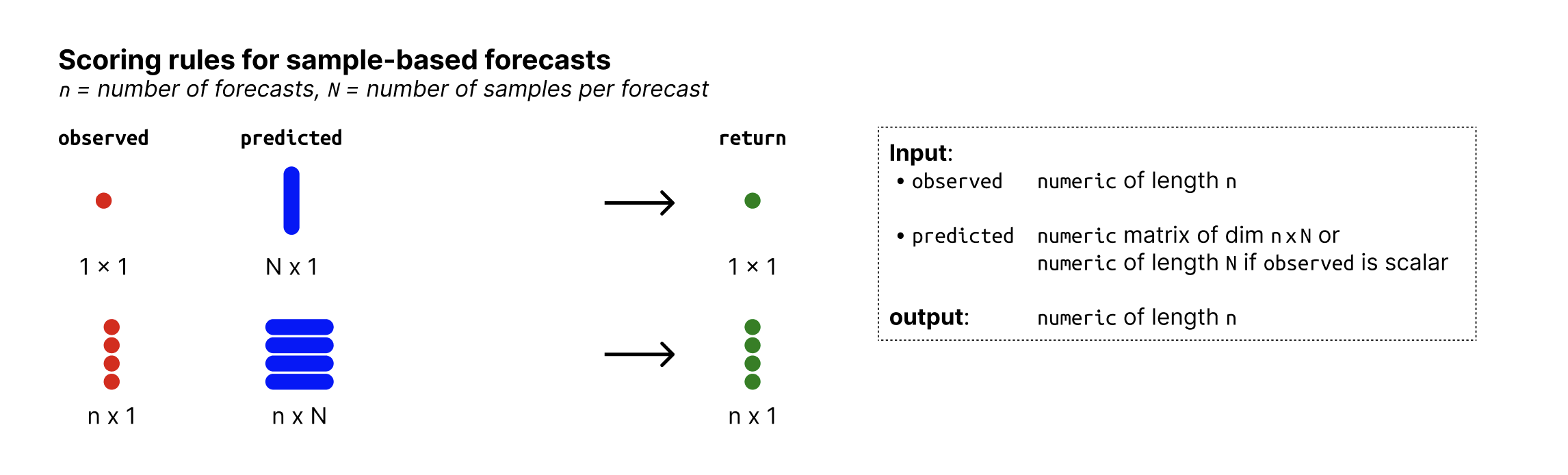
Numeric vector of length n with the biases of the predictive samples with respect to the observed values.
Details
For continuous forecasts, Bias is measured as
$$ B_t (P_t, x_t) = 1 - 2 * (P_t (x_t)) $$
where \(P_t\) is the empirical cumulative distribution function of the prediction for the observed value \(x_t\). To handle ties appropriately (which can occur when predictions equal observations for exampele due to rounding), \(P_t(x_t)\) is computed using mid-ranks: the fraction of predictive samples strictly smaller than \(x_t\) plus half the fraction equal to \(x_t\).
For integer valued forecasts, Bias is measured as
$$ B_t (P_t, x_t) = 1 - (P_t (x_t) + P_t (x_t + 1)) $$
to adjust for the integer nature of the forecasts.
In both cases, Bias can assume values between -1 and 1 and is 0 ideally.
References
The integer valued Bias function is discussed in Assessing the performance of real-time epidemic forecasts: A case study of Ebola in the Western Area region of Sierra Leone, 2014-15 Funk S, Camacho A, Kucharski AJ, Lowe R, Eggo RM, et al. (2019) Assessing the performance of real-time epidemic forecasts: A case study of Ebola in the Western Area region of Sierra Leone, 2014-15. PLOS Computational Biology 15(2): e1006785. doi:10.1371/journal.pcbi.1006785
Examples
## integer valued forecasts
observed <- rpois(30, lambda = 1:30)
predicted <- replicate(200, rpois(n = 30, lambda = 1:30))
bias_sample(observed, predicted)
#>  [1]  0.660 -0.025  0.710 -0.930  0.870  0.435 -0.885 -0.940 -0.515 -0.790
#> [11]  0.975 -0.975 -0.620 -0.740 -0.640  0.395  0.695 -0.765 -0.935 -0.680
#> [21] -0.725 -0.320  0.355  0.730  0.250  0.995 -0.650  0.235  0.250  0.850

## continuous forecasts
observed <- rnorm(30, mean = 1:30)
predicted <- replicate(200, rnorm(30, mean = 1:30))
bias_sample(observed, predicted)
#>  [1] -0.46  0.02  0.02  0.12 -0.18 -0.07  0.96 -0.60  0.16 -0.31  0.79  0.49
#> [13] -0.74 -0.48  0.26 -0.56  0.82  0.89  0.41 -0.31  0.19  0.47 -0.85  0.32
#> [25]  0.15 -0.16  0.34 -0.30  0.80  0.27