Plot Contributions to the Weighted Interval Score

Visualise the components of the weighted interval score: penalties for over-prediction, under-prediction and for high dispersion (lack of sharpness)

Usage

plot_wis(scores, x = "model", relative_contributions = FALSE, flip = FALSE)

Arguments

scores: A data.frame of scores based on quantile forecasts as produced by score() and summarised using summarise_scores()
x: The variable from the scores you want to show on the x-Axis. Usually this will be "model".
relative_contributions: show relative contributions instead of absolute contributions. Default is FALSE and this functionality is not available yet.
flip: boolean (default is FALSE), whether or not to flip the axes.

Value

A ggplot2 object showing a contributions from the three components of the weighted interval score

References

Bracher J, Ray E, Gneiting T, Reich, N (2020) Evaluating epidemic forecasts in an interval format. https://journals.plos.org/ploscompbiol/article?id=10.1371/journal.pcbi.1008618

Examples

library(ggplot2)
scores <- score(example_quantile)
#> The following messages were produced when checking inputs:
#> 1.  144 values for `prediction` are NA in the data provided and the corresponding rows were removed. This may indicate a problem if unexpected.
scores <- summarise_scores(scores, by = c("model", "target_type"))

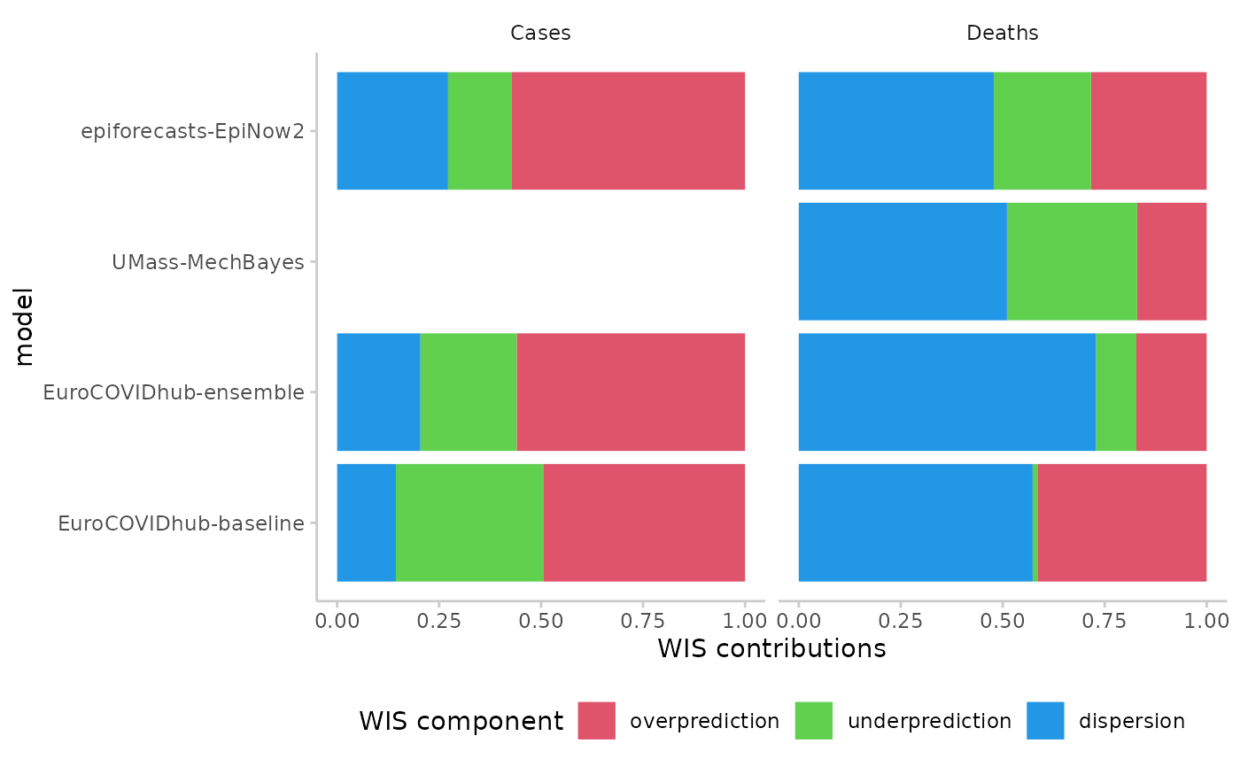
plot_wis(scores,
  x = "model",
  relative_contributions = TRUE
) +
  facet_wrap(~target_type)

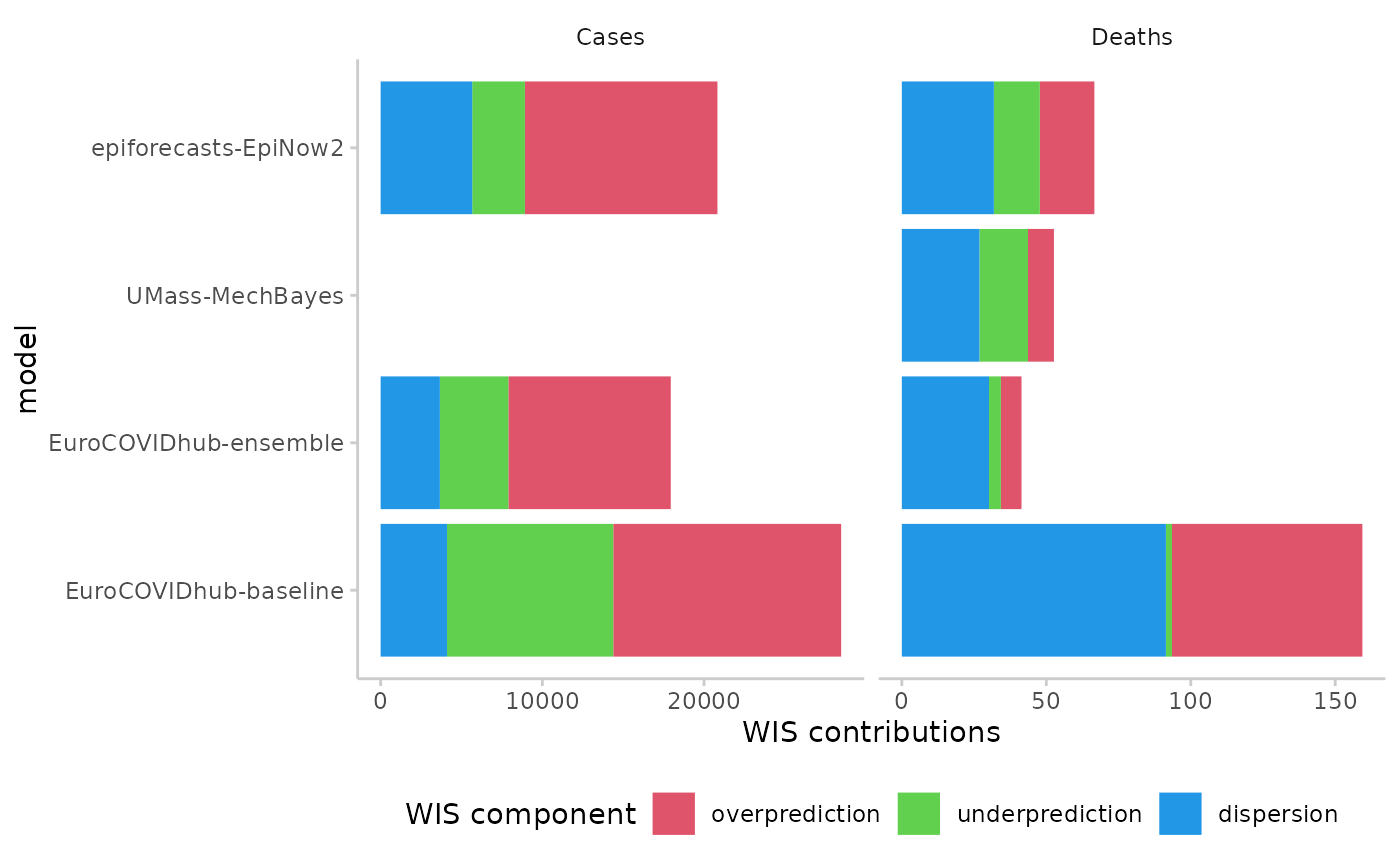
plot_wis(scores,
  x = "model",
  relative_contributions = FALSE
) +
  facet_wrap(~target_type, scales = "free_x")