DiagrammeR::grViz('
digraph processes {
  graph [rankdir = TB, fontname = "inherit", bgcolor = "white"]
  node  [shape = box, style = filled, fillcolor = "white",
         color = "black", fontcolor = "black", fontname = "inherit"]
  edge  [color = "black"]

  subgraph cluster_FG {
    label = "Forecast-generating process"; color = "black"; fontcolor = "black"
    F1 [label = "Model specification"]
    F2 [label = "Model implementation"]
    F3 [label = "Forecaster participation"]
  }
  subgraph cluster_TG {
    label = "Target-generating process"; color = "black"; fontcolor = "black"
    T1 [label = "Epidemic dynamics"]
    T2 [label = "Target observation"]
    T3 [label = "Target specification"]
  }
  F [label = "Prediction"]
  T [label = "Target"]
  P [label = "Forecast performance"]

  F1 -> F; F2 -> F; F3 -> F
  F -> P
  T1 -> T; T2 -> T; T3 -> T
  T -> P
}
')Interpreting variation in infectious disease forecast performance with model-based evaluation
Katharine Sherratt (1), Rok Grah (2), Bastian Prasse (2), Friederike Becker (3), Jamie McLean (1), Sam Abbott (1), Sebastian Funk (1)
- Centre for Mathematical Modelling of Infectious Diseases, London School of Hygiene & Tropical Medicine
- European Centre for Disease Prevention and Control
- Institute of Statistics, Karlsruhe Institute of Technology
Email: katharine.sherratt@.ac.uk
Caution
Under development
Abstract
Forecasters predicting infectious disease outbreaks meet with varying success. When many forecasters each predict many different targets, it is difficult to identify why their performance varies. Considering this variation, we separate the process of creating a forecast from the process generating the target it predicts. Comparing across combinations of the two conflates the method a forecaster used with the difficulty of the targets they chose, while stratifying by these factors leaves too few comparable forecasts. We identify common strategies for this problem, and demonstrate a regression-based approach to evaluation with sparse data.
We evaluated 207,713 forecasts of weekly COVID-19 cases and deaths from 48 models over two years across 32 European countries, scored against observed data with the weighted interval score of log-transformed values (LWIS). We classified models by structure (agent-based, mechanistic, semi-mechanistic, statistical, or human judgement), and estimated the effect of model structure in a generalised additive mixed model adjusting for the epidemiological outcome, its level and trend, the dominant pathogen variant, the country, the forecast horizon, whether a model forecast for one or many countries, and differences between individual models. No model structure was clearly different from the overall average (ratios 0.96 to 1.08 of the average LWIS, all intervals spanning 1). Instead, performance was driven by factors varying between forecast targets, such as the epidemic trend. We left substantial variation in individual model performance unexplained. When ranking individual models by their performance relative to others in the sample, we noted an individual model’s ordinal position was only weakly persistent before-and-after adjustment (Spearman’s rank correlation 0.37).
Our model-based approach sits between informal and fully formal ways of handling bias in observational studies of forecast performance. Less formal designs such as stratification suffice with a single target or a structured sample of forecasters, while going further could include propensity weighting or a fully specified causal estimand. As infectious disease forecasting grows, we encourage evaluators to match the formality of the design to the question and the data available. Evaluating across multiple forecast targets requires explicit accounting for the variation producing each target, before considering what varies within the forecasting process.
Main text
Background
Forecasters predicting infectious disease outbreaks meet with varying success. This variation is increasingly visible as the field adopts standardised methods for evaluating and comparing forecasts. This presents an opportunity to investigate the correlates and causes of variation in forecast performance. We suggest that two separate processes contribute to realised forecast performance: those that contribute to producing a forecast, and those that generate the observed target for prediction (Figure 1). Distinguishing between these separates the room for improvement available to a forecasting method, from the accuracy that can be expected from any forecast in a given infectious disease setting.
Identifying the relative impact of these factors requires many independent forecasters predicting many differing targets, and comparably scored for resulting accuracy. Participatory forecast challenges aim to provide this by collating predictions for pre-specified targets in a standardised format, with forecasters free to choose which targets they predict [1,2]. Nonetheless, this creates two problems for evaluation. Repeated forecasts from the same model are not independent, so evaluating across them risks becoming overpowered by the number of forecasts, yet underpowered to detect differences between models (akin to pseudoreplication [3]). Further, comparisons that are aggregated across targets conflate the performance of model structure with the specific difficulty of different epidemiological targets for prediction.
Evidence on factors within the forecasting process is unclear. As in many forecasting domains, the only reliably strong performance has come from ensemble combinations of many forecasters [4–6]. Individual forecasters use approaches ranging from purely data-driven statistical models, to mechanistic models embedding explicit hypotheses about transmission, and these structures suit different purposes, such as scenario projection, policy analysis, or nowcasting [7–9]. Some evaluations find better performance from statistical over more mechanistic model structures [10–12], while others have repeatedly found little evidence that any structure performs better than another [13–15]. Model structure is the most consistently recorded aspect of the forecasting process. Other factors in model specification and implementation are rarely or inconsistently documented in enough detail to support comparison.
Factors producing variation among forecast targets are somewhat better understood. Performance is better under stable epidemic dynamics [16], in larger populations [17], where surveillance is timely and accurate [15,18], and where informative leading indicators exist [10]. Predictive difficulty also varies systematically between pathogens and between seasons of the same pathogen [19]. Performance is consistently better at shorter forecast horizons [5], and for outcomes with longer delays from infection to report, such as for deaths compared to cases [4]. Because forecasters choose which targets to predict, these factors can confound any comparison between models or model structures, making such comparisons hard to interpret.
Evaluation is particularly difficult where forecasts must be cross-classified by several of these sources at once. Even a large set of forecasts becomes sparse once stratified by several covariates, leaving too few forecasts in each stratum to estimate a stable and unbiased association (“sparse-data bias” [20]). Traditional methods from observational research offer varying degrees of formality in controlling which units are compared [3,21,22]; Table 1.
| Threat to validity | Approach to control | Example use in forecast evaluation | Limitation |
|---|---|---|---|
| None | Unadjusted comparison | Rank models, or compare summary scores, over all forecasts as submitted | Conflates the method used with the difficulty of the targets each model chose to forecast |
| Confounding, selection | Inclusion criteria | Exclude forecasts without comparable reporting of probabilistic uncertainty [4] | Loses power; narrows the population the estimate applies to |
| Confounding | Matching on covariates | Compare forecasters only on targets both submitted for [23] | Sparse overlap; the estimate holds only for the matched set |
| Confounding | Stratification | Report scores by horizon, location, or epidemic phase [5,15] | Cells sparse and uneven with several interacting factors; continuous covariates need arbitrary binning |
| Differential population sizes | Indirect standardisation | Relative skill against a naive baseline model available for all targets [23] | Interpretable only against the chosen reference, which materially changes rankings [24] |
| Confounding, clustering | Regression adjustment | Estimate the partial effect of model structure, adjusting for the covariates of the target | Specification-dependent; the estimand is not formally defined |
Here we develop one approach to tracing specific influences on forecast performance, while accounting for variation across the forecast- and target-generating processes. We use a joint estimation regression approach that makes use of all observations to inform each estimate, rather than discarding those outside a stratum or matched set. We demonstrate this with forecasts from 48 models predicting short-term COVID-19 incidence across Europe, and focus on the effect of model structure on performance. We classified models into five categories of model structure, and adjusted for other features of the forecasting process and target. We found performance was more strongly associated with the forecast target than with model structure. We interpret this in the context of study designs for comparative forecast evaluation, and propose directions for more detailed comparative evaluations.
Methods
Study design
We aimed to estimate the effect of model structure on forecast performance. We evaluated forecasts of incident COVID-19 cases and deaths for 32 European countries between 8 March 2021 and 10 March 2023, collected by the public European COVID-19 Forecast Hub [25]. The Hub solicited real-time forecasts one to four weeks ahead. Any forecaster was eligible for inclusion, with no selection criteria. For this analysis, we excluded forecasts that did not report the full set of 23 quantiles or that were more than four weeks ahead. Models could forecast any subset of the four horizons, noting that 8 of 48 did not forecast all four. We also excluded the ensemble of all Hubs models. Full eligibility and a STROBE flow diagram are given in the Supplement.
We evaluated forecasts against Johns Hopkins University data on cumulative daily reported cases and deaths [26], converted to incident weekly counts, as available on 10 March 2023 when collation stopped. Before evaluation, we normalised forecasts and observations to incidence per 100,000 population and log-transformed both. This supports comparability across varying populations with varying magnitude of incidence across locations and over time. The log-transform can also be read as evaluating prediction of the growth rate [27].
We scored forecasts with the weighted interval score (WIS), a proper scoring rule and generalisation of the continuous ranked probability score, reflecting a forecast’s dispersion, overprediction and underprediction [23]. We report this log-transformed data evaluated with the WIS as the LWIS, and separately report the natural-scale WIS in the Supplement.
Forecasting processes
We classified model structures as “Agent-based” (detailed individual-level interactions), “Mechanistic” (broadly compartmental), “Semi-mechanistic” (statistical models with epidemiological elements such as delay distributions or generation intervals), “Statistical” (context-agnostic time-series), and “Judgement” (ensembles of human-judgement predictions). Classification used self-reported metadata: an optional description of methods, and links to model code, website or publication (schema and example in the Supplement). Four of us (KS, SF, FB, JM) classified models independently, with at least two rating each model. The majority vote determined the final classification, ties were resolved by an additional independent rater, and two investigators (SF, KS) reviewed all classifications.
We classified each model as forecasting for a single country or for more than one, using a binary classification (“CountryTargets”) rather than a count of countries because few models submitted for between 2 and 32 countries, and because forecasters changed the number of targets they submitted over time. A random effect for individual model identity separates the contribution of model structure from variation between individual implementations.
Epidemiological target processes
We include two epidemiological outcomes, incident cases or deaths, and considered these to separately interact with the effect of model structure. We then considered observed data associated with our view of important transmission dynamics. Upstream of transmission, we include the target country, as a proxy for population-level transmission behaviour and policy; and dominant circulating pathogen variant, classified from public sequence data into a discrete sequence of phases [28]. Downstream of transmission, we identified the count of incident outcomes in the target week, and the trend of incidence (“Stable”, “Increasing” or “Decreasing”, from a three-week moving average (with a change of +/-5% as “Stable”). We fully detail each included covariate in the Supplement.
Residual confounding
We include the length of forecast horizon (from 1 to 4 weeks) as a common confounding variable representing increasing uncertainty of forecasting further ahead; we allow this effect to vary for each individual model.
We did not adjust for unobserved characteristics of the forecasting team, such as capacity, infrastructure, or experience, although these plausibly shape both the choice of model structure and realised performance. We therefore treat the estimand as a direct rather than a total effect, considering possible unmeasured confounders. We illustrate our approach as a directed acyclic graph in the Supplement, and consider this work exploratory rather than fully causal.
Model-based analysis
We fitted a single hierarchical model across both epidemiological outcomes. The LWIS is continuous, non-negative and strongly right-skewed, so we treated the LWIS of each forecast \(i\) as Tweedie-distributed with a log link, letting the linear predictor \(\eta_i\) act multiplicatively on the expected score:
\[ \mathrm{LWIS}_i \sim \mathrm{Tw}_p(\mu_i,\, \phi), \qquad \log \mu_i = \eta_i, \]
where \(\phi\) is the dispersion and the power parameter \(p \in (1, 2)\) is estimated alongside the smoothing parameters, giving a variance function \(\mathrm{Var}(\mathrm{LWIS}_i) = \phi\,\mu_i^{p}\). We adopted a Tweedie distribution to support forecasts scoring exactly zero. We compared this against a Gaussian and a Gamma on the same specification (see Supplement). The estimated \(p\) was 1.93, close to a Gamma, but a Gamma has no support at zero and would require an arbitrary constant for these scores.
The linear predictor decomposed into a fixed intercept, a fixed effect for the epidemiological outcome, random-effect contributions from categorical covariates, and two smooths for continuous covariates:
\[ \eta_i = \beta_0 \;+\; \beta_{\text{outcome}}\,\mathbb{1}[\text{Deaths}_i] \;+\; \underbrace{\sum_{g \in \mathcal{G}} u^{g}_{j_g(i)}}_{\text{random effects}} \;+\; \underbrace{f_{\text{Inc}}(\mathrm{Incidence}_i) \;+\; f_{\text{Horizon}}(\mathrm{Horizon}_i) \;+\; f^{\text{Horizon}}_{k(i)}(\mathrm{Horizon}_i)}_{\text{smooths}}. \]
Here \(\beta_{\text{outcome}}\) gives the deaths-versus-cases contrast on the log scale (cases as reference) and is not part of the zero-mean Gaussian random-effects set \(\mathcal{G}\), and \(j_g(i)\) denotes the level of grouping factor \(g\) for forecast \(i\):
\[ u^{g}_{j} \sim \mathcal{N}(0,\, \sigma^2_g), \qquad g \in \mathcal{G} = \{\text{Method} \times \text{Outcome},\, \text{CountryTargets},\, \text{Trend},\, \text{Variant},\, \text{Location}\}. \]
Model structure enters as a single grouping factor crossing with epidemiological outcome, giving one effect per cell, so a structure may predict cases relatively better than deaths or the reverse. We report both the separate effects per outcome and the pooled effect of each structure as a contrast averaging its two cells, which accounts for the covariance between them. The epidemiological outcome remains a fixed effect. Being unpenalised, this absorbs any difference common to all structures, leaving the crossed term to carry variation from it. Both choices are set out in the Supplement.
\(f_{\text{Inc}}\) was a penalised thin-plate regression spline over log-transformed incidence. Forecast performance is known to worsen with horizon, so \(f_{\text{Horizon}}\) was a smooth of horizon shared by all models. Each model \(k\) had its own deviation from this curve, \(f^{\text{Horizon}}_k\), with its level and slope penalised towards zero. Both smooths used four basis functions. We compare alternative horizon specifications in the Supplement.
We fitted all models with the mgcv package in R using fast restricted maximum likelihood [29]. We checked fit by visual inspection of residuals and conducted extensive sensitivity analysis. To assess confounding, we also fitted univariate models to provide a comparison between unadjusted and adjusted estimates of the effect of model structure on LWIS. We report each categorical effect as the exponentiated random effect, which multiplies the expected LWIS relative to the population mean (a zero random effect), with all other terms held fixed; the epidemiological outcome is reported as deaths relative to cases. A ratio of 0.9 represents an expected LWIS 10% lower (better) than the population mean. We report each individual model’s effect as its average deviation from the shared horizon curve over the horizons for which that model forecast. We report raw partial effects in the Supplement.
All data and code are publicly available online [30].
Results
We evaluated 48 forecasting models from 38 modelling teams participating in the European COVID-19 Forecast Hub over 2021-2023.
Participant characteristics
| Characteristic | Cases N = 91 |
Cases & Deaths N = 341 |
Deaths N = 51 |
All included, N = 481 |
|---|---|---|---|---|
| Model structure | ||||
| Agent-based | 1 (11%) | 2 (5.9%) | 0 (0%) | 3 (6.3%) |
| Judgement | 0 (0%) | 3 (8.8%) | 0 (0%) | 3 (6.3%) |
| Mechanistic | 1 (11%) | 15 (44%) | 1 (20%) | 17 (35%) |
| Semi-mechanistic | 2 (22%) | 7 (21%) | 3 (60%) | 12 (25%) |
| Statistical | 5 (56%) | 7 (21%) | 1 (20%) | 13 (27%) |
| Participation (%) | 1.4 (0.4, 2.9) | 3.1 (1.9, 24.0) | 2.1 (2.1, 2.8) | 2.9 (1.5, 13.7) |
| 1 n (%); Median (Q1, Q3) | ||||
Forecasters could participate in any of 26,624 available targets (104 weeks, 32 countries, 4 horizons, 2 epidemiological outcomes). Among them, forecasters covered 98% of available targets, with a median of 8 models forecasting each covered target (IQR 6-9, maximum 22). Coverage was uneven across countries, weeks and model structures (Supplement). Median participation was 3% of available targets (IQR 2-13%, range 0 to 98).
We classified 17 models as mechanistic, 13 as statistical, 12 as semi-mechanistic, 3 as agent-based and 3 as human judgement (Table 2; Supplement). Raters disagreed on 17 (35%) classifications, most often for semi-mechanistic models, 8 of which drew one vote for a statistical structure. Statistical models contributed the largest share of predictions (41%), partly because the Hub baseline model submitted for every country in almost every week. Mechanistic and semi-mechanistic models contributed 30% and 28%, and agent-based and judgement models under 2% each.
Forecast performance
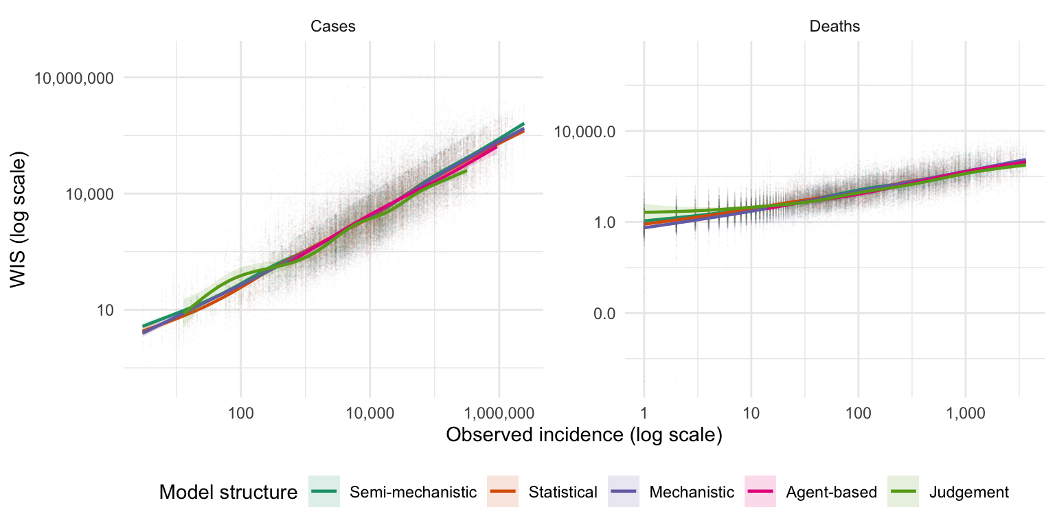
Aggregated performance varied with the epidemiological outcome, its magnitude, the variant phase and the forecast horizon. Case forecasts scored a median LWIS of 0.29 against 0.10 for deaths. For deaths in particular, scores varied non-linearly with the magnitude of the outcome being predicted (Figure 2). Across variant phases, forecasts were most accurate during the Delta phase and least accurate during Omicron-BA.1, the period of steepest change in reported incidence. Scores worsened with forecast horizon (Figure 2), from a median LWIS of 0.14 at one week to 0.52 at four weeks for cases, and 0.07 to 0.14 for deaths. Against the Hub ensemble, constructed from the median of the forecasts we assess in this analysis, 15 of 43 models achieved a lower median LWIS for cases (ensemble 0.21) and 17 of 39 for deaths (ensemble 0.07).
Effect of model structure
Participation between model structures was unevenly distributed across forecast targets. To assess the sparse-data problem for these forecasts, we cross-classified them by epidemiological outcome, forecast horizon, location, epidemic trend, variant phase, single or multiple countries, and model structure. This gives 46,080 possible strata, of which 30% contain any forecast. Among these, each non-empty stratum holds a median of only 10 forecasts and 24% hold fewer than five.
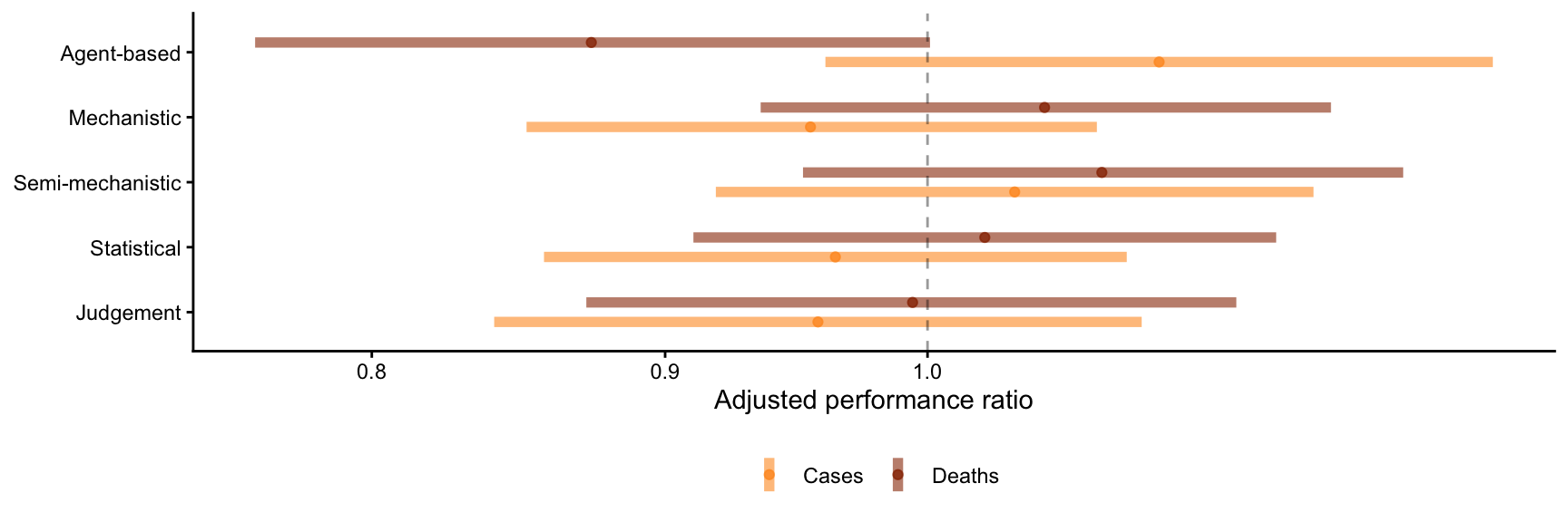
After adjustment, no model structure was clearly different from the average (Table 3, Figure 3). The largest shifts under adjustment were among agent-based and human judgement models, while adjustment shrank the standard errors throughout.
| Variable | Group | Unadjusted ratio (95% CI) | Adjusted ratio (95% CI) |
|---|---|---|---|
| Method | Agent-based | 0.86 (0.7, 1.05) | 0.97 (0.86, 1.1) |
| Judgement | 0.74 (0.61, 0.9) | 0.96 (0.86, 1.08) | |
| Mechanistic | 1.09 (0.9, 1.32) | 0.99 (0.9, 1.09) | |
| Semi-mechanistic | 1.22 (1.01, 1.47) | 1.08 (0.98, 1.2) | |
| Statistical | 1.18 (0.97, 1.42) | 0.99 (0.9, 1.09) |
Differences between model structures were modified by epidemiological outcome (Figure 3; Supplement). The widest separation was among agent-based models, which were the worst-performing model structure for case forecasts but the best for death forecasts (cases ratio 1.09 (0.95-1.25); deaths ratio 0.87 (0.75-1.00)), while their pooled estimate sits close to the average. This contrast rests on 3 models and 814 forecasts for cases, and 2 models and 720 forecasts for deaths, so the structure-level estimate is close to a statement about individual models, even with a model-specific effect in the fit.
Other model structures performed more similarly between epidemiological outcomes, performing marginally better on cases than on deaths. Differences between outcomes largely offset in the pooled estimate for each structure.
Wider influences on forecast performance
Epidemiological processes generating the forecast target explained more variation in performance than features of the forecasting process. Performance was best during stable periods of the epidemic curve (ratio 0.79 (0.61-1.01)) and worst during increasing trends (ratio 1.21 (0.94-1.55)). Performance was better in the earlier Alpha and Delta phases (ratios 0.82 (0.72-0.94) and 0.81 (0.71-0.93)) and worst under Omicron BA.1 (ratio 1.22 (1.06-1.39)), and death forecasts scored lower than case forecasts (ratio 0.35 (0.31-0.40)). We report the total set of modelled effects in the Supplement.
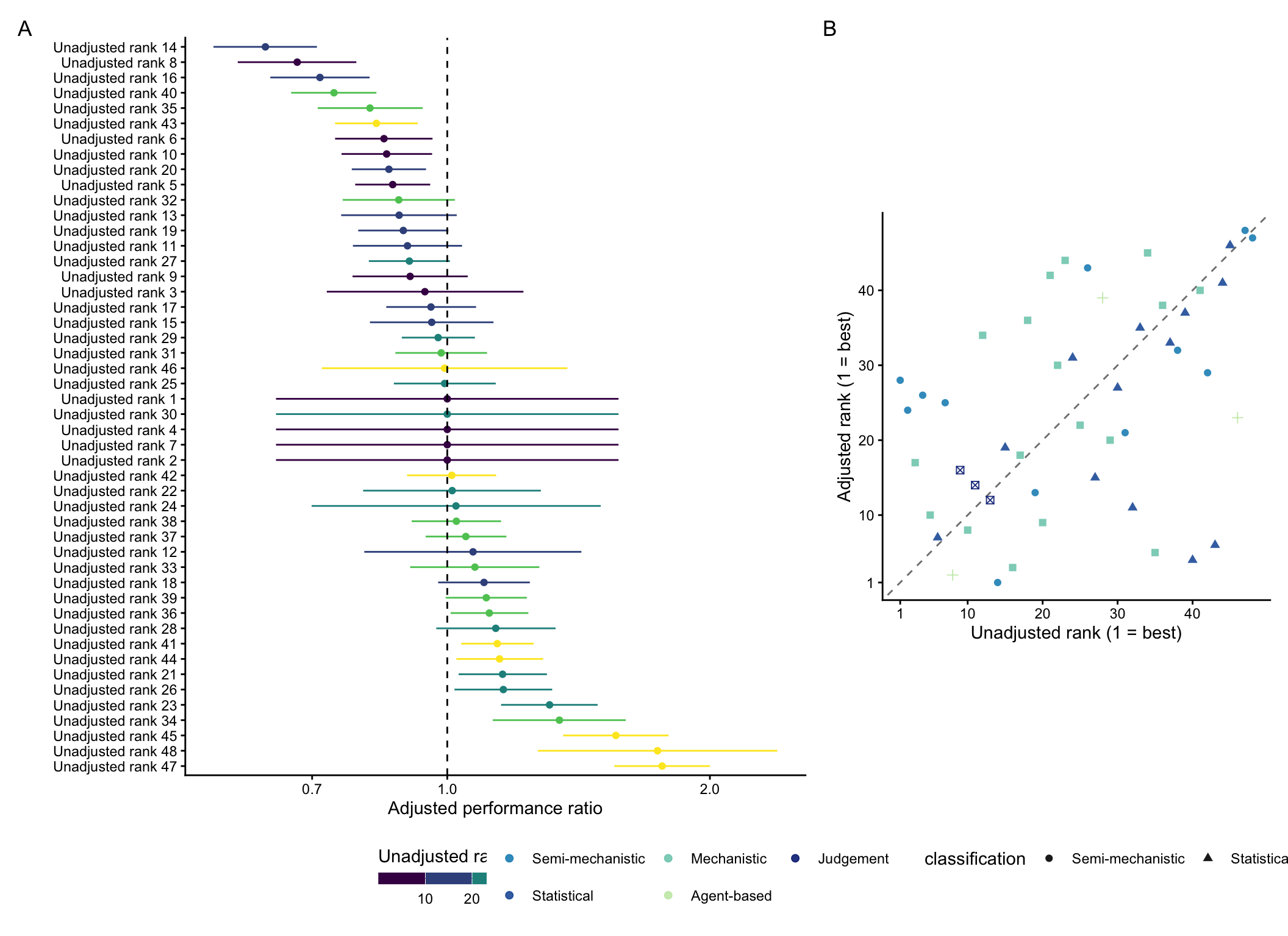
Most of the difference between individual model performance was left unexplained (Figure 4 A). We accounted for whether models forecast for one or multiple countries, with 19 models forecasting for a single country and 29 for multiple countries (of which only 2 kept the same number of countries throughout, see Supplement). Both estimates were shrunk to the average (single-country ratio 1.00 (1.00-1.00); multi-country ratio 1.00 (1.00-1.00)), explaining none of the difference between models. We specified the effect of forecast horizon as a single shared curve among all models, from which each model deviated in its own set of forecast horizons.
We compared this remaining variation between individual models in terms of ranked model order. Ranking models by their performance before and after adjustment gives a Spearman correlation of 0.37. 18 of 48 models moved at least 10 places, with the furthest moving 41 places (Figure 4 B).
Sensitivity analysis
Repeating the analysis on the natural scale gave the same direction for each structure, but semi-mechanistic models performed more consistently worse than average (ratio 1.57, 1.04–2.35) (Supplement). The exception was the choice of error family: refitting with a Gaussian in place of the Tweedie changed the size of every structure-by-outcome estimate and the direction of two of the five. Specifically, this widened the case-death difference for human judgement models, removed it for agent-based models, and reversed it for semi-mechanistic models.
Discussion
We grouped 48 models forecasting COVID-19 across European countries into five model structures, and estimated the effect of structure jointly with variation among forecasters and among the targets each predicted. No structure was distinguishable from the overall average, while individual forecasters’ performance varied substantially. Predictive performance depended more on the difficulty of the target than on the structure of the forecasting model. Fair comparison across forecasters and targets therefore requires accounting for confounding between these processes.
With an effective sample of 48 independent models, we found no clear evidence that any of the five model structures performed better than the others. This agrees with evaluations that found no consistent difference between structures [13–15], and does not reproduce the advantage for statistical structures reported in forecasting challenges for chikungunya, influenza and dengue [10–12]. Those evaluations covered other pathogens and settings, which may explain part of the difference. Our results point to a further explanation: individual model rankings changed substantially once we accounted for prediction target. Differences between outcomes also largely offset within each structure, and a pooled estimate near the average does not rule out a structure performing better for one outcome than the other. The instability in individual rankings did not relate to model structure, which suggests that for a given forecast target, forecasters have as much to learn from models unlike their own as from those sharing their structure.
Features of the epidemiological target instead made substantial differences to performance. This is consistent with evidence that particular pathogens and seasons are intrinsically harder to forecast than others [31], and with concerns that the complexity of infectious disease dynamics limits predictability. The turning point and end of an expanding epidemic may not be precisely forecastable [32], and predictability itself is bounded, more tightly for endemic-epidemic outbreaks than for others [33]. Where the target sets much of the error, the room left for a forecasting method to improve is smaller than an unadjusted comparison implies.
Forecast hubs typically rank models by relative skill against a baseline model [23], an indirect standardisation whose rankings depend on the chosen reference [24]. We found that rankings also shifted when adjusting for the targets each model predicted. Public health agencies selecting or weighting individual models by their past performance should treat rankings from unadjusted comparisons with caution [4,5].
A model-based evaluation of this kind is extremely flexible. We developed the specification here over several iterations and do not consider it final. There are likely many additional interactions between the effects explored here. For example, different model structures may be more or less well equipped to predict at each interval of the one to four week forecast horizon; those able to incorporate underlying epidemic mechanisms may be less responsive to shorter term data artefacts but relatively better able to demonstrate the impact of longer term dynamics. We allowed each individual model its own deviation from a shared horizon curve, which may have absorbed these structural differences. We also only partially accounted for variation among forecast targets. For example, real-time data were frequently updated retrospectively, with different frequencies and magnitudes between national surveillance and reporting systems [18], so the target a forecast was scored against was not always the target available when it was made. Nonetheless, varying the inclusion of some covariates and the link function left the effects of model structure essentially unchanged (see Supplement). The error family mattered more: a Gaussian fit changed the size of every structure-by-outcome estimate and the direction of two, as it is dominated by the largest scores, which fall disproportionately among case forecasts. Any single structure-by-outcome contrast should be read with this sensitivity in mind.
Two further sources of bias follow from the observational design. We had no information on how forecasters chose which targets to predict and when to participate, so we could only adjust for the observed features of those targets. If forecasters joined, paused or stopped in response to unmeasured factors, such as how well their own model had recently performed, the adjusted estimates remain biased. We also did not adjust for unobserved characteristics of forecasting teams, such as capacity, infrastructure, or experience, which plausibly shape both the choice of model structure and performance, and we therefore estimate a direct effect of structure. While the model-specific random effect separates structure from other stable differences between models, it cannot remove confounding where those differences are correlated with structure.
We adopted a coarse characterisation of the forecasting process, while a more sophisticated view could point towards interventions to improve forecast accuracy. We pre-specified five structures by their inclusion of mechanism, but we had little access to model metadata, raters disagreed on most semi-mechanistic models, and we did not track changes to each model’s methods over time. Our findings also come from a single pathogen, collaborative project, and set of two outcomes over two years in Europe, and we did not test whether the same balance between target and method holds elsewhere. Combining several collaborative efforts would increase the sample of independent models, enough to assess finer components of the forecasting process, such as the effect of forecasters’ resources, capacity, or motivation. Future comparison projects could support this by encouraging methodological diversity, and collating structured metadata, such as methodology and model revisions, alongside predictions [1].
Clarifying how performance relates to the scale and scope of human involvement in model development, implementation, or validation deserves specific focus. Generally stronger performance has been linked to forecasters’ experience and capacity to anticipate underlying data-generating processes, such as changing surveillance, behaviour, or pathogen characteristics [11,16,34]. In this study, we also noted strong unadjusted differences in models using greater levels of human involvement, whether this was encoded qualitatively (human judgement forecasters)[35], or quantitatively (agent-based models)[36]. However, these contributed 6/48 forecasting models and under 5% of predictions. With so few models, an estimate for one of these structures is close to a statement about the individual models it contains, even with a model-specific effect in the fit. Our framework used penalised terms, shrinking such sparsely informed cells towards the null, so the wide intervals here plausibly reflect uncertainty from few independent models, not necessarily greater true variability in performance. Hubs could deliberately recruit and record forecasters’ use of judgement, which would also inform forecasting with human-in-the-loop large language models.
We conclude that the choice of evaluation design is not neutral for interpreting variation in forecast performance. As the field of infectious disease forecasting develops, greater investment [37] and standardisation [38,39] are creating a broader comparable sample of forecast performance. This reduces random error when comparing models. However, by itself this increase in size cannot account for bias in the sample of either forecasters or forecast targets. We consider our model-based approach here a middle ground among formal methods for handling bias. Less formality, such as simple stratification, may suffice with minimal confounding among forecast targets (e.g. a single target), or with a more structured sample of forecasters (e.g. quota-based). Adding formality to address differential participation could include propensity score methods, to weight each forecast by the probability that its model submitted for that target [22]. Going further still, a fully specified causal estimand could include describing both forecast-generating and target-generating processes, deriving a minimal sufficient adjustment set [40], and identifying unmeasured confounding with quantitative bias analysis [41]. Rather than defaulting to any one of these, we encourage evaluators to match the formality of the study design to the intended generality of the hypothesis.
References
1.
Pollett S, Johansson M, Biggerstaff M, Morton LC, Bazaco SL, Brett-Major DM, et al. Identification and evaluation of epidemic prediction and forecasting reporting guidelines: A systematic review and a call for action. Epidemics. 2020;33: 100400. doi:10.1016/j.epidem.2020.100400
2.
Reich NG, Lessler J, Funk S, Viboud C, Vespignani A, Tibshirani RJ, et al. Collaborative hubs: Making the most of predictive epidemic modeling. American Journal of Public Health. 2022;112: 839–842. doi:10.2105/ajph.2022.306831
3.
Heffner RA, Butler MJ, Reilly CK. Pseudoreplication revisited. Ecology. 1996;77: 2558–2562.
4.
Sherratt K, Gruson H, Grah R, Johnson H, Niehus R, Prasse B, et al. Predictive performance of multi-model ensemble forecasts of COVID-19 across european nations. eLife. 2023;12: e81916. doi:10.7554/eLife.81916
5.
Cramer EY, Ray EL, Lopez VK, Bracher J, Brennen A, Castro Rivadeneira AJ, et al. Evaluation of individual and ensemble probabilistic forecasts of COVID-19 mortality in the united states. Proceedings of the National Academy of Sciences. 2022;119: e2113561119. doi:10.1073/pnas.2113561119
6.
Reich NG, McGowan CJ, Yamana TK, Tushar A, Ray EL, Osthus D, et al. Accuracy of real-time multi-model ensemble forecasts for seasonal influenza in the u.s. PLOS Computational Biology. 2019;15: e1007486. doi:10.1371/journal.pcbi.1007486
7.
Woolhouse M. How to make predictions about future infectious disease risks. Philosophical Transactions of the Royal Society B: Biological Sciences. 2011;366: 2045–2054. doi:10.1098/rstb.2010.0387
8.
Dattner I, Huppert A. Modern statistical tools for inference and prediction of infectious diseases using mathematical models. Statistical Methods in Medical Research. 2018;27: 1927–1929. doi:10.1177/0962280217746456
9.
Funk S, King AA. Choices and trade-offs in inference with infectious disease models. Epidemics. 2020;30: 100383. doi:10.1016/j.epidem.2019.100383
10.
Del Valle SY, McMahon BH, Asher J, Hatchett R, Lega JC, Brown HE, et al. Summary results of the 2014-2015 DARPA chikungunya challenge. BMC Infectious Diseases. 2018;18: 245. doi:10.1186/s12879-018-3124-7
11.
McGowan CJ, Biggerstaff M, Johansson M, Apfeldorf KM, Ben-Nun M, Brooks L, et al. Collaborative efforts to forecast seasonal influenza in the united states, 2015–2016. Scientific Reports. 2019;9: 683. doi:10.1038/s41598-018-36361-9
12.
Johansson MA, Apfeldorf KM, Dobson S, Devita J, Buczak AL, Baugher B, et al. An open challenge to advance probabilistic forecasting for dengue epidemics. Proceedings of the National Academy of Sciences. 2019;116: 24268–24274.
13.
Carlson CJ, Dougherty E, Boots M, Getz W, Ryan SJ. Consensus and conflict among ecological forecasts of zika virus outbreaks in the united states. Scientific Reports. 2018;8: 4921. doi:10.1038/s41598-018-22989-0
14.
Viboud C, Sun K, Gaffey R, Ajelli M, Fumanelli L, Merler S, et al. The RAPIDD ebola forecasting challenge: Synthesis and lessons learnt. Epidemics. 2018;22: 13–21. doi:10.1016/j.epidem.2017.08.002
15.
Reich NG, Brooks LC, Fox SJ, Kandula S, McGowan CJ, Moore E, et al. A collaborative multiyear, multimodel assessment of seasonal influenza forecasting in the united states. Proceedings of the National Academy of Sciences. 2019;116: 3146–3154. doi:10.1073/pnas.1812594116
16.
Bracher J, Wolffram D, Deuschel J, Görgen K, Ketterer JL, Ullrich A, et al. National and subnational short-term forecasting of COVID-19 in germany and poland during early 2021. Communications Medicine. 2022;2: 1–17. doi:10.1038/s43856-022-00191-8
17.
Lopez VK, Cramer EY, Pagano R, Drake JM, O’Dea EB, Adee M, et al. Challenges of COVID-19 case forecasting in the US, 2020–2021. PLOS Computational Biology. 2024;20: e1011200. doi:10.1371/journal.pcbi.1011200
18.
Holcomb KM, Mathis S, Staples JE, Fischer M, Barker CM, Beard CB, et al. Evaluation of an open forecasting challenge to assess skill of west nile virus neuroinvasive disease prediction. Parasites & Vectors. 2023;16: 11.
19.
Metcalf CJE, Mahmud AS, Grenfell BT. Comparative dynamics, seasonality in transmission, and predictability of childhood infections in mexico. Epidemiology and Infection. 2017;145: 607–625. doi:10.1017/S0950268816002673
20.
Greenland S, Mansournia MA, Altman DG. Sparse data bias: A problem hiding in plain sight. BMJ. 2016;352: i1981. doi:10.1136/bmj.i1981
21.
McNamee R. Regression modelling and other methods to control confounding. Occupational and Environmental Medicine. 2005;62: 500–506. doi:10.1136/oem.2002.001115
22.
Kahlert J, Gribsholt SB, Gammelager H, Dekkers OM, Luta G. Control of confounding in the analysis phase — an overview for clinicians. Clinical Epidemiology. 2017;9: 195–204. doi:10.2147/CLEP.S129886
23.
Bracher J, Ray EL, Gneiting T, Reich NG. Evaluating epidemic forecasts in an interval format. PLOS Computational Biology. 2021;17: e1008618. doi:10.1371/journal.pcbi.1008618
24.
Stapper M, Funk S. Mind the baseline: The hidden impact of reference model selection on forecast assessment. medRxiv; 2025. doi:10.1101/2025.08.01.25332807
25.
European COVID-19 Forecast Hub. European COVID-19 forecast hub. https://covid19forecasthub.eu/; 2021.
26.
Dong E, Du H, Gardner L. An interactive web-based dashboard to track COVID-19 in real time. The Lancet Infectious Diseases. 2020;20: 533–534. doi:10.1016/s1473-3099(20)30120-1
27.
Bosse NI, Abbott S, Cori A, Leeuwen E van, Bracher J, Funk S. Scoring epidemiological forecasts on transformed scales. PLOS Computational Biology. 2023;19: e1011393. doi:10.1371/journal.pcbi.1011393
28.
European Centre for Disease Prevention and Control. SARS-CoV-2 variants of concern. https://www.ecdc.europa.eu/en/covid-19/variants-concern; 2023.
29.
Wood SN. Fast stable restricted maximum likelihood and marginal likelihood estimation of semiparametric generalized linear models. Journal of the Royal Statistical Society: Series B (Statistical Methodology). 2011;73: 3–36. doi:10.1111/j.1467-9868.2010.00749.x
30.
Sherratt K, Funk S. Epiforecasts/eval-by-method: v0.1.0. Zenodo; 2025. doi:10.5281/zenodo.14903162
31.
White LA, León TM. Forecastability of infectious disease time series: Are some seasons and pathogens intrinsically more difficult to forecast? medRxiv. 2025. doi:10.1101/2025.04.29.25326677
32.
Castro M, Ares S, Cuesta JA, Manrubia S. The turning point and end of an expanding epidemic cannot be precisely forecast. Proceedings of the National Academy of Sciences. 2020;117: 26190–26196. doi:10.1073/pnas.2007868117
33.
Scarpino SV, Petri G. On the predictability of infectious disease outbreaks. Nature Communications. 2019;10: 898. doi:10.1038/s41467-019-08616-0
34.
Clapham H, Gad M, Gheorghe A, Hutubessy R, Megiddo I, Painter C, et al. Assessing fitness-for-purpose and comparing the suitability of COVID-19 multi-country models for local contexts and users. Gates Open Research. 2021. doi:10.12688/gatesopenres.13224.1
35.
Bosse NI, Abbott S, Bracher J, Leeuwen E van, Cori A, Funk S. Human judgement forecasting of COVID-19 in the UK. Wellcome Open Research. 2024;8: 416. doi:10.12688/wellcomeopenres.19380.2
36.
Wolffram D, Abbott S, Heiden M an der, Funk S, Günther F, Hailer D, et al. Collaborative nowcasting of COVID-19 hospitalization incidences in germany. PLOS Computational Biology. 2023;19: e1011394. doi:10.1371/journal.pcbi.1011394
37.
Rivers C, Chretien J-P, Riley S, Pavlin JA, Woodward A, Brett-Major D, et al. Using "outbreak science" to strengthen the use of models during epidemics. Nature Communications. 2019;10: 3102. doi:10.1038/s41467-019-11067-2
38.
Pollett S, Johansson MA, Reich NG, Brett-Major D, Del Valle SY, et al. Recommended reporting items for epidemic forecasting and prediction research: The EPIFORGE 2020 guidelines. PLOS Medicine. 2021;18: e1003793. doi:10.1371/journal.pmed.1003793
39.
Kerr M, Borchering R, Castro Rivadeneira A, Contamin L, Funk S, Hochheiser H, et al. A software platform for collaborative infectious disease modeling. medRxiv; 2025. doi:10.1101/2025.10.03.25337284
40.
Hernán MA, Robins JM. Causal inference: What if. Boca Raton: Chapman & Hall/CRC; 2020. Available: https://miguelhernan.org/whatifbook
41.
VanderWeele TJ, Ding P. Sensitivity analysis in observational research: Introducing the e-value. Annals of Internal Medicine. 2017;167: 268–274. doi:10.7326/M16-2607
Supporting Information
S1 Text. Supplementary methods, results and sensitivity analyses. Contains: sources of forecast and observed data, and study participation, with the eligibility flow diagram and the characteristics of contributing models; derivation of the epidemic trend and variant phase covariates; the causal diagram and covariate selection, the specification of the structure-by-outcome term, and model fitting with the comparison of error families; partial effects for every covariate, the raw partial effects on the log scale, structure-by-outcome estimates, and the models whose rank changes most under adjustment; and sensitivity analyses covering population normalisation, the natural-scale score, covariate selection, the error family, and structure-by-outcome estimates under a Gaussian family.
Data availability
The codebase for this paper is publicly available at the Github repository “epiforecasts/eval-by-method” and Zenodo with DOI: 10.5281/zenodo.14903162. Forecast and observed data were sourced from the European COVID-19 Forecast Hub, available to view online. All Hub data are now archived at the Github repository: “european-modelling-hubs/covid19-forecast-hub-europe_archive” and Zenodo with DOI: 10.5281/zenodo.13986751. Specific data used in this work are available in the Github repository for this paper.