This supplement supports “Using model-based evaluation to interpret variation in infectious disease forecast performance”. It is organised as the analysis runs: how forecasts and observations were sourced and who took part; how the covariates were derived; how the model was specified and fitted; the full set of estimates behind the main-text figures; and the sensitivity analyses. Every number and figure here is generated from the same fitted model as the main text, output/log/results.rds.
Methods
Source data and code
Forecast and observed data were sourced from the European COVID-19 Forecast Hub, available to view at https://covid19forecasthub.eu/ . All Hub data are now archived at:
- Github: https://github.com/european-modelling-hubs/covid19-forecast-hub-europe_archive
- Zenodo with DOI: https://doi.org/10.5281/zenodo.13986751
Data for this work were downloaded on 30th May 2023. These data are available in the Github repository for this paper at: https://github.com/epiforecasts/eval-by-method/tree/main/data
The codebase for this paper is publicly available at:
- Github: https://github.com/epiforecasts/eval-by-method
- Zenodo with DOI: https://doi.org/10.5281/zenodo.14903162
Comments and code contributions are welcome - please use Github Issues.
Please cite code using:
- Katharine Sherratt & Sebastian Funk. (2025). epiforecasts/eval-by-method: Zenodo. https://doi.org/10.5281/zenodo.14903162
Study participation
Forecasting teams were recruited to the European Covid-19 Forecast Hub using existing networks and ECDC publicity. Any forecaster was eligible to participate, and there were no selection criteria. All participation was voluntary and unrenumerated. Forecasters contributed a standard set of metadata describing their team and model, and uploaded forecasts weekly. Forecasters were optionally able to express uncertainty by reporting a distribution of up to 23 probabilistic quantiles for each prediction. Forecasts were validated against minimal formatting requirements for quantile intervals and that values were positive integers.
For this study, we collected all forecasts from between 8 March 2021 to 10 March 2023. We excluded forecasts of hospitalisations, which experienced multiple changes in source data during the study period. We excluded forecasts that did not report the full set of 23 quantiles, in order to ensure fair comparison among probabilistic model results. We also excluded the ensemble model created by the Hub team, because it is constructed from the contributed forecasts and so would double-count them. We retained the Hub baseline model: it is an independently specified statistical model, and including it gives a naive reference point against which participant forecasts can be read.
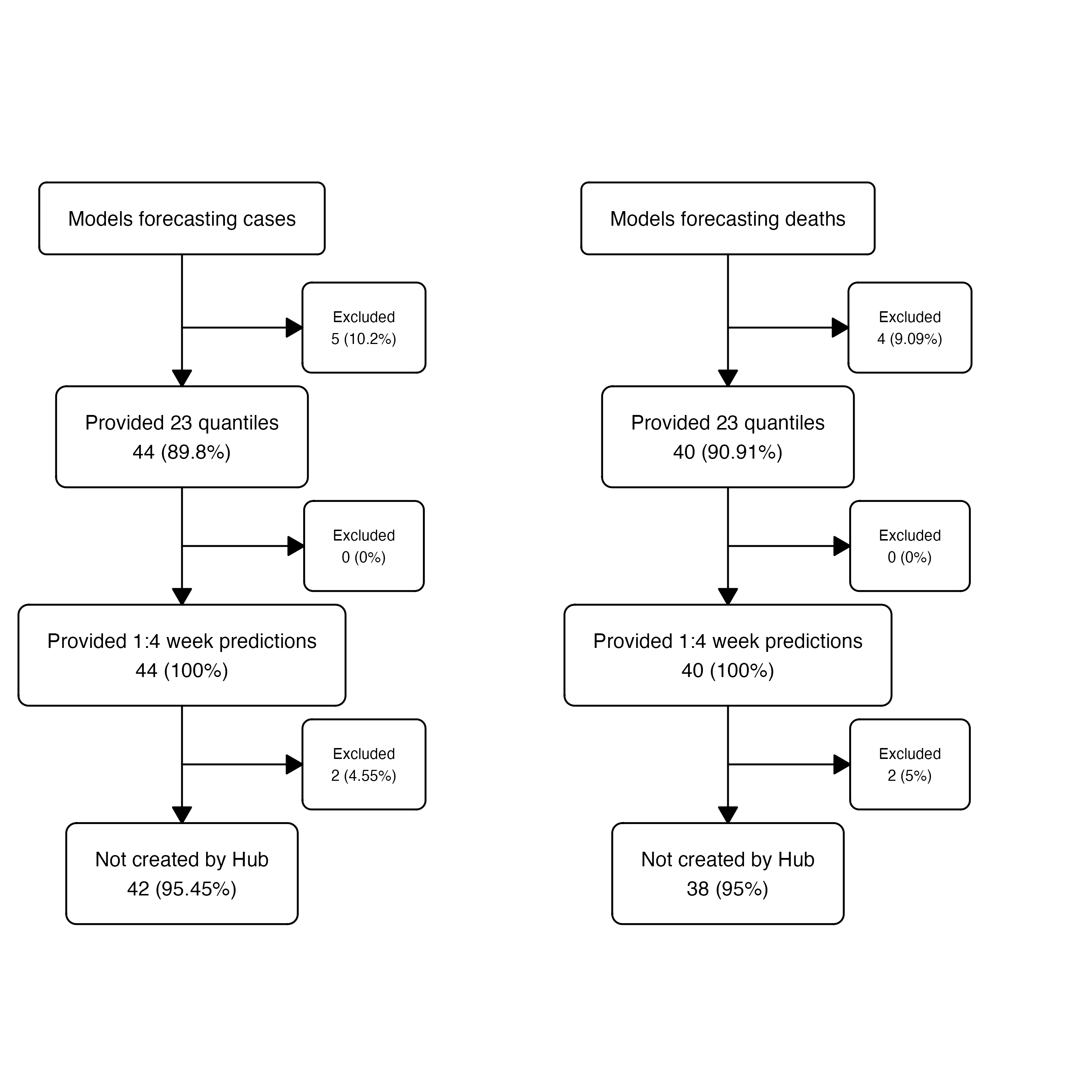
Of 49 models submitting case forecasts during the study period, 43 met these criteria; of 44 submitting death forecasts, 39 did.
Characteristics of contributing models:
| Model | Method | Country Targets | Case forecasts | Death forecasts |
|---|---|---|---|---|
| AMM-EpiInvert | Statistical | Multi-country | 2,788 | |
| CovidMetrics-epiBATS | Statistical | Single-country | 343 | |
| DSMPG-bayes | Semi-mechanistic | Multi-country | 760 | |
| EuroCOVIDhub-baseline | Statistical | Multi-country | 13,082 | 13,040 |
| FIAS_FZJ-Epi1Ger | Mechanistic | Single-country | 264 | 264 |
| GoeWroc-BaseBayes | Semi-mechanistic | Single-country | 12 | |
| HZI-AgeExtendedSEIR | Mechanistic | Single-country | 382 | 382 |
| ICM-agentModel | Agent-based | Single-country | 334 | 334 |
| IEM_Health-CovidProject | Mechanistic | Multi-country | 7,710 | 7,708 |
| ILM-EKF | Semi-mechanistic | Multi-country | 11,998 | 11,961 |
| ITWW-county_repro | Semi-mechanistic | Multi-country | 650 | 600 |
| Imperial-DeCa | Semi-mechanistic | Multi-country | 571 | |
| Imperial-RtI0 | Semi-mechanistic | Multi-country | 571 | |
| Imperial-sbkp | Semi-mechanistic | Multi-country | 571 | |
| JBUD-HMXK | Mechanistic | Multi-country | 1,324 | 1,324 |
| KITmetricslab-bivar_branching | Statistical | Single-country | 8 | |
| Karlen-pypm | Mechanistic | Multi-country | 3,208 | 3,186 |
| LANL-GrowthRate | Semi-mechanistic | Multi-country | 3,692 | 3,696 |
| LeipzigIMISE-SECIR | Mechanistic | Single-country | 16 | 16 |
| MIMUW-StochSEIR | Mechanistic | Single-country | 76 | 76 |
| MIT_CovidAnalytics-DELPHI | Mechanistic | Multi-country | 348 | 500 |
| MOCOS-agent1 | Agent-based | Single-country | 386 | 386 |
| MUNI-ARIMA | Statistical | Multi-country | 10,979 | 11,314 |
| MUNI-LaggedRegARIMA | Statistical | Multi-country | 736 | |
| MUNI-VAR | Statistical | Multi-country | 976 | 976 |
| MUNI_DMS-SEIAR | Mechanistic | Single-country | 224 | 200 |
| PL_GRedlarski-DistrictsSum | Mechanistic | Single-country | 378 | |
| RobertWalraven-ESG | Statistical | Multi-country | 9,190 | 10,465 |
| SDSC_ISG-TrendModel | Statistical | Multi-country | 1,756 | 1,744 |
| UB-BSLCoV | Statistical | Single-country | 96 | 96 |
| UC3M-EpiGraph | Agent-based | Single-country | 94 | |
| ULZF-SEIRC19SI | Mechanistic | Single-country | 249 | 249 |
| UMass-MechBayes | Mechanistic | Multi-country | 5,948 | |
| UMass-SemiMech | Semi-mechanistic | Multi-country | 1,888 | 1,904 |
| UNED-PreCoV2 | Statistical | Single-country | 147 | 147 |
| UNIPV-BayesINGARCHX | Statistical | Multi-country | 426 | |
| USC-SIkJalpha | Mechanistic | Multi-country | 12,900 | 12,688 |
| UpgUmibUsi-MultiBayes | Semi-mechanistic | Single-country | 99 | 99 |
| bisop-seirfilter | Mechanistic | Single-country | 32 | 32 |
| bisop-seirfilterlite | Mechanistic | Multi-country | 336 | 336 |
| epiMOX-SUIHTER | Mechanistic | Single-country | 134 | 134 |
| epiforecasts-EpiExpert | Judgement | Multi-country | 945 | 948 |
| epiforecasts-EpiExpert_Rt | Judgement | Multi-country | 404 | 404 |
| epiforecasts-EpiExpert_direct | Judgement | Multi-country | 394 | 392 |
| epiforecasts-EpiNow2 | Semi-mechanistic | Multi-country | 8,843 | 7,721 |
| epiforecasts-weeklygrowth | Statistical | Multi-country | 5,971 | |
| itwm-dSEIR | Mechanistic | Single-country | 406 | 406 |
| prolix-euclidean | Semi-mechanistic | Multi-country | 800 | 800 |
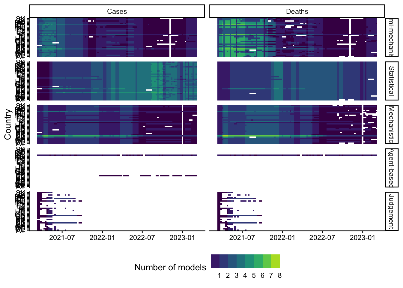
Number of models participating in forecasting 1-week ahead case incidence for each country over the study period.
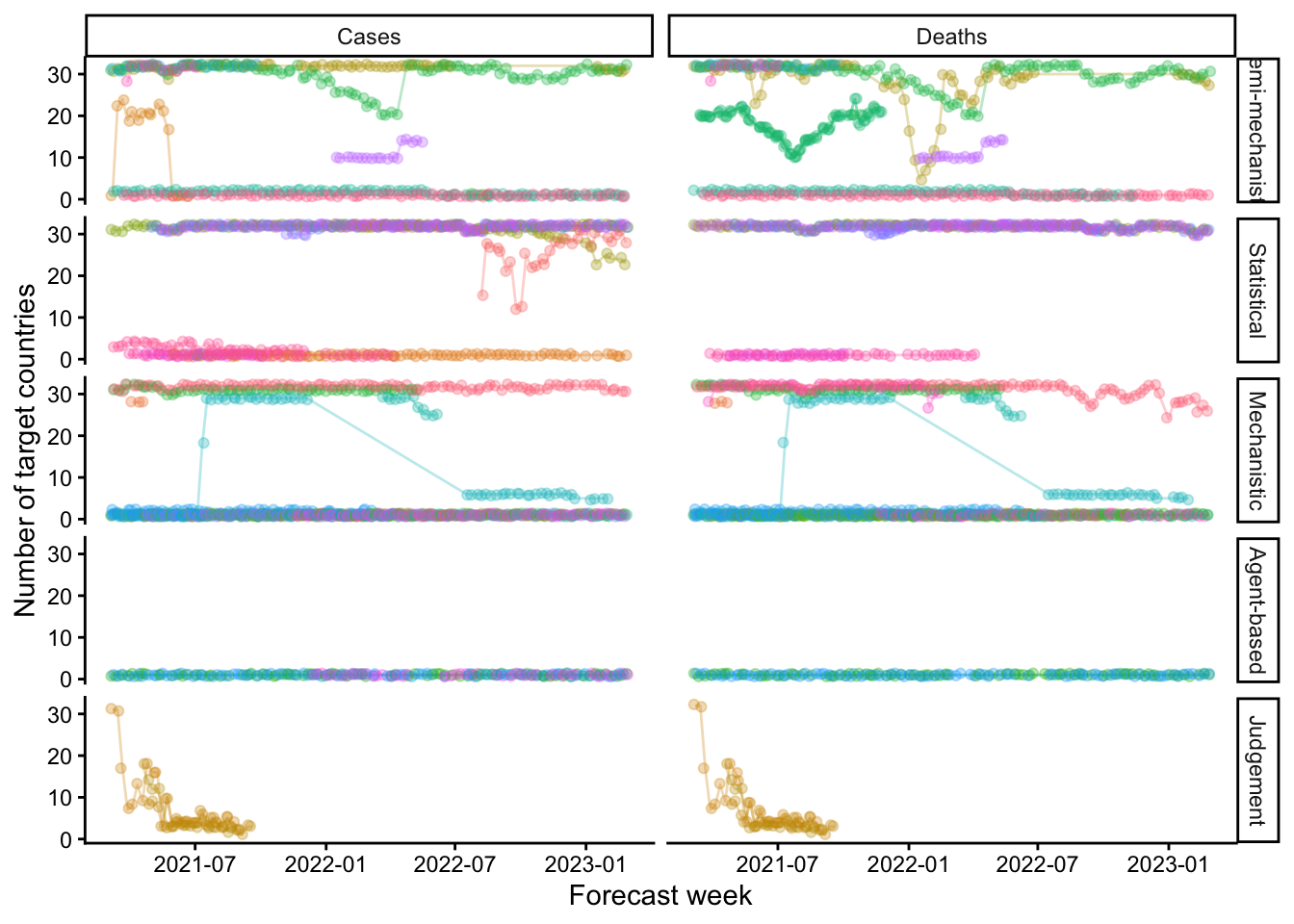
We explored how models selected geographic targets over time. Forecasters both added and removed targets among the set for which they forecast each week. This figure shows number of targets submitted by each model at the 1-week ahead horizon. We noted the same variation for 2-4 week forecasts.
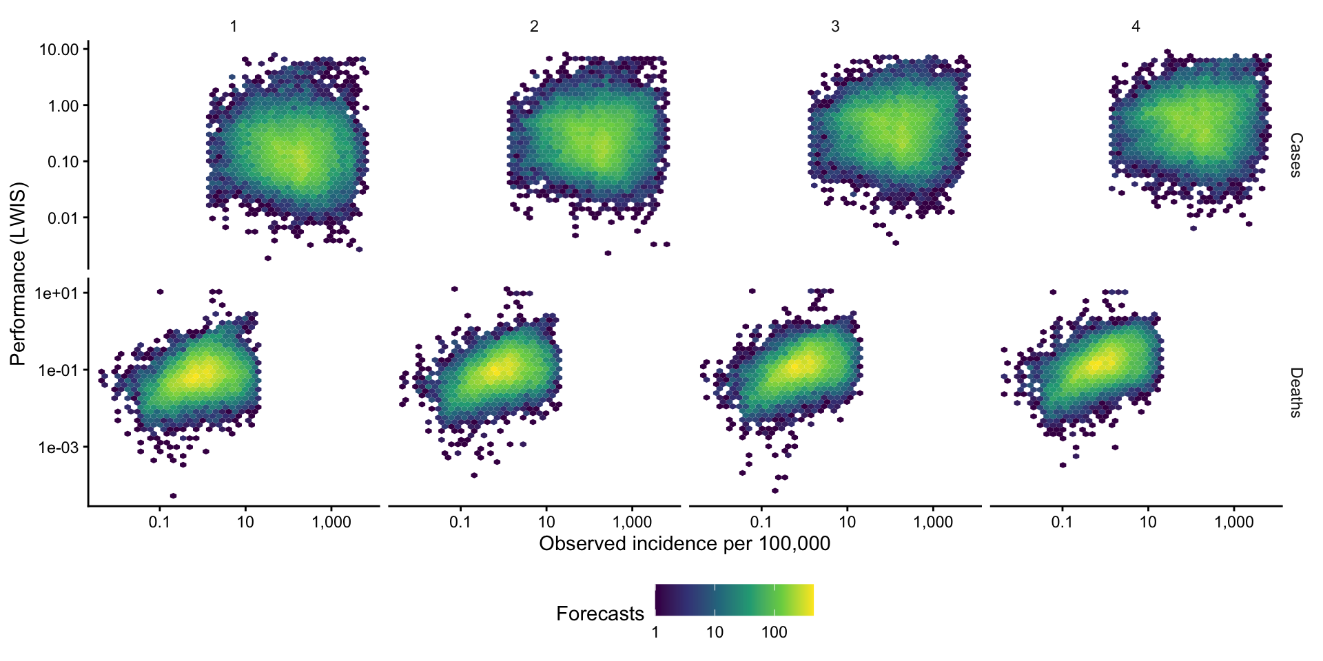
The main text shows this same relationship as aggregated percentile bands. At the level of individual forecasts, the same data show where forecasts actually concentrate and where scores cluster or trail off.
Data processing
Model structure classification
Human raters classified models according to methodological structures.
| Model | Final classification | Agreement | Total raters | Semi-mechanistic | Mechanistic | Agent-based | Statistical | Judgement | Other | Machine Learning |
|---|---|---|---|---|---|---|---|---|---|---|
| AMM-EpiInvert | Statistical | FALSE | 3 | 0 | 0 | 0 | 2 | 0 | 1 | 0 |
| DSMPG-bayes | Semi-mechanistic | FALSE | 3 | 2 | 0 | 0 | 1 | 0 | 0 | 0 |
| ILM-EKF | Semi-mechanistic | FALSE | 3 | 2 | 0 | 0 | 1 | 0 | 0 | 0 |
| ITWW-county_repro | Semi-mechanistic | FALSE | 3 | 2 | 0 | 0 | 1 | 0 | 0 | 0 |
| Imperial-DeCa | Semi-mechanistic | FALSE | 3 | 2 | 0 | 0 | 1 | 0 | 0 | 0 |
| Imperial-RtI0 | Semi-mechanistic | FALSE | 3 | 2 | 0 | 0 | 1 | 0 | 0 | 0 |
| Imperial-sbkp | Semi-mechanistic | FALSE | 3 | 2 | 0 | 0 | 1 | 0 | 0 | 0 |
| KITmetricslab-bivar_branching | Statistical | FALSE | 3 | 1 | 0 | 0 | 2 | 0 | 0 | 0 |
| Karlen-pypm | Mechanistic | FALSE | 3 | 0 | 2 | 0 | 1 | 0 | 0 | 0 |
| LANL-GrowthRate | Semi-mechanistic | FALSE | 3 | 2 | 0 | 0 | 1 | 0 | 0 | 0 |
| SDSC_ISG-TrendModel | Statistical | FALSE | 3 | 0 | 0 | 0 | 2 | 0 | 1 | 0 |
| UMass-SemiMech | Semi-mechanistic | FALSE | 4 | 3 | 1 | 0 | 0 | 0 | 0 | 0 |
| USC-SIkJalpha | Mechanistic | FALSE | 4 | 1 | 3 | 0 | 0 | 0 | 0 | 0 |
| UpgUmibUsi-MultiBayes | Semi-mechanistic | FALSE | 3 | 2 | 0 | 0 | 1 | 0 | 0 | 0 |
| bisop-seirfilter | Mechanistic | FALSE | 4 | 1 | 3 | 0 | 0 | 0 | 0 | 0 |
| bisop-seirfilterlite | Mechanistic | FALSE | 4 | 1 | 3 | 0 | 0 | 0 | 0 | 0 |
| prolix-euclidean | Semi-mechanistic | FALSE | 4 | 3 | 0 | 0 | 0 | 0 | 1 | 0 |
| CovidMetrics-epiBATS | Statistical | TRUE | 3 | 0 | 0 | 0 | 3 | 0 | 0 | 0 |
| EuroCOVIDhub-baseline | Statistical | TRUE | 4 | 0 | 0 | 0 | 4 | 0 | 0 | 0 |
| FIAS_FZJ-Epi1Ger | Mechanistic | TRUE | 3 | 0 | 3 | 0 | 0 | 0 | 0 | 0 |
| GoeWroc-BaseBayes | Semi-mechanistic | TRUE | 3 | 3 | 0 | 0 | 0 | 0 | 0 | 0 |
| HZI-AgeExtendedSEIR | Mechanistic | TRUE | 3 | 0 | 3 | 0 | 0 | 0 | 0 | 0 |
| ICM-agentModel | Agent-based | TRUE | 3 | 0 | 0 | 3 | 0 | 0 | 0 | 0 |
| IEM_Health-CovidProject | Mechanistic | TRUE | 4 | 0 | 4 | 0 | 0 | 0 | 0 | 0 |
| JBUD-HMXK | Mechanistic | TRUE | 3 | 0 | 3 | 0 | 0 | 0 | 0 | 0 |
| LeipzigIMISE-SECIR | Mechanistic | TRUE | 3 | 0 | 3 | 0 | 0 | 0 | 0 | 0 |
| MIMUW-StochSEIR | Mechanistic | TRUE | 3 | 0 | 3 | 0 | 0 | 0 | 0 | 0 |
| MIT_CovidAnalytics-DELPHI | Mechanistic | TRUE | 3 | 0 | 3 | 0 | 0 | 0 | 0 | 0 |
| MOCOS-agent1 | Agent-based | TRUE | 3 | 0 | 0 | 3 | 0 | 0 | 0 | 0 |
| MUNI-ARIMA | Statistical | TRUE | 3 | 0 | 0 | 0 | 3 | 0 | 0 | 0 |
| MUNI-LaggedRegARIMA | Statistical | TRUE | 3 | 0 | 0 | 0 | 3 | 0 | 0 | 0 |
| MUNI-VAR | Statistical | TRUE | 3 | 0 | 0 | 0 | 3 | 0 | 0 | 0 |
| MUNI_DMS-SEIAR | Mechanistic | TRUE | 3 | 0 | 3 | 0 | 0 | 0 | 0 | 0 |
| PL_GRedlarski-DistrictsSum | Mechanistic | TRUE | 3 | 0 | 3 | 0 | 0 | 0 | 0 | 0 |
| RobertWalraven-ESG | Statistical | TRUE | 3 | 0 | 0 | 0 | 3 | 0 | 0 | 0 |
| UB-BSLCoV | Statistical | TRUE | 3 | 0 | 0 | 0 | 3 | 0 | 0 | 0 |
| UC3M-EpiGraph | Agent-based | TRUE | 3 | 0 | 0 | 3 | 0 | 0 | 0 | 0 |
| ULZF-SEIRC19SI | Mechanistic | TRUE | 3 | 0 | 3 | 0 | 0 | 0 | 0 | 0 |
| UMass-MechBayes | Mechanistic | TRUE | 3 | 0 | 3 | 0 | 0 | 0 | 0 | 0 |
| UNED-PreCoV2 | Statistical | TRUE | 3 | 0 | 0 | 0 | 3 | 0 | 0 | 0 |
| UNIPV-BayesINGARCHX | Statistical | TRUE | 3 | 0 | 0 | 0 | 3 | 0 | 0 | 0 |
| epiMOX-SUIHTER | Mechanistic | TRUE | 3 | 0 | 3 | 0 | 0 | 0 | 0 | 0 |
| epiforecasts-EpiExpert | Judgement | TRUE | 3 | 0 | 0 | 0 | 0 | 3 | 0 | 0 |
| epiforecasts-EpiExpert_Rt | Judgement | TRUE | 3 | 0 | 0 | 0 | 0 | 3 | 0 | 0 |
| epiforecasts-EpiExpert_direct | Judgement | TRUE | 3 | 0 | 0 | 0 | 0 | 3 | 0 | 0 |
| epiforecasts-EpiNow2 | Semi-mechanistic | TRUE | 3 | 3 | 0 | 0 | 0 | 0 | 0 | 0 |
| epiforecasts-weeklygrowth | Statistical | TRUE | 2 | 0 | 0 | 0 | 2 | 0 | 0 | 0 |
| itwm-dSEIR | Mechanistic | TRUE | 3 | 0 | 3 | 0 | 0 | 0 | 0 | 0 |
Epidemic trend identification
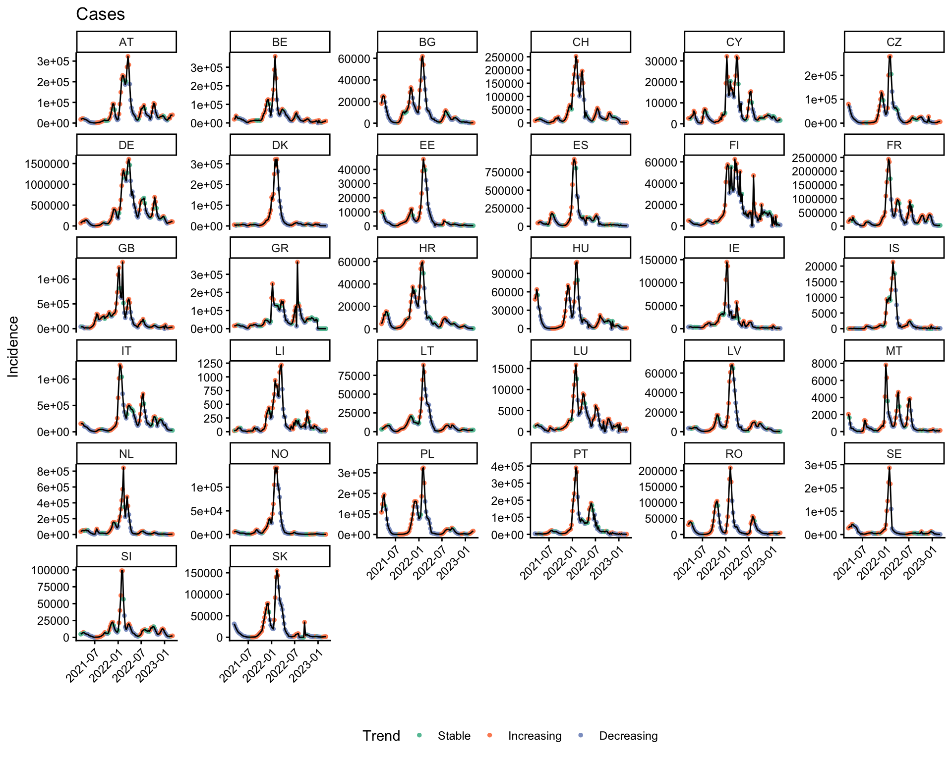
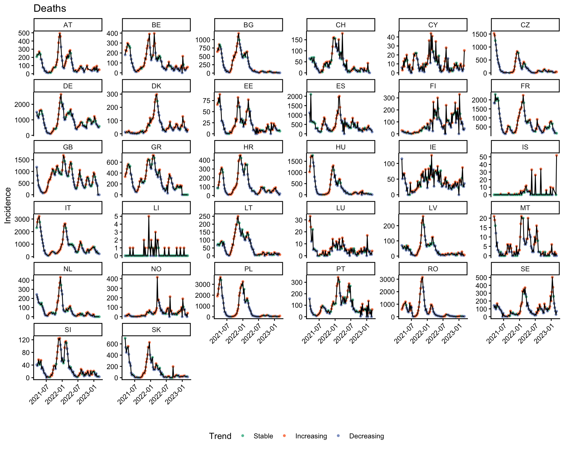
We categorised each week as “Stable”, “Decreasing”, or “Increasing”, based on the difference over a three-week moving average of incidence (with a change of +/-5% as “Stable”).
Variant phase identification
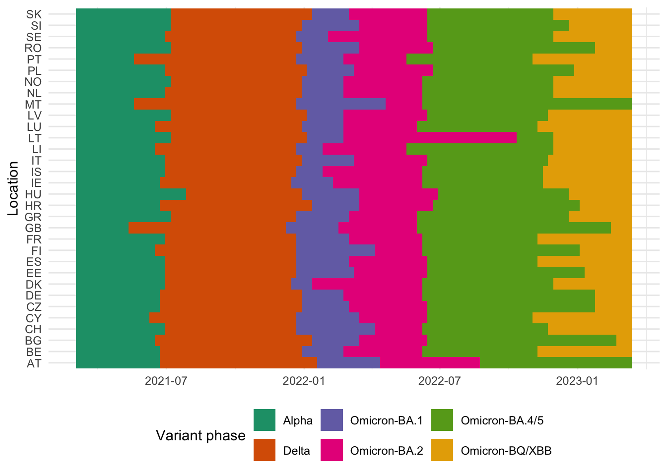
Genomic surveillance data were obtained from three sources: ECDC (covering 30 European countries), UKHSA (Great Britain), and the Swiss Federal Office of Public Health (Switzerland). Variant lineages were mapped to six named phases in expected chronological order: Alpha, Delta, Omicron-BA.1, Omicron-BA.2, Omicron-BA.4/5, and Omicron-BQ/XBB. For each country, we identified the first week in which each named variant exceeded 50% of sequenced samples. We enforced chronological ordering by removing any out-of-sequence phases, then expanded phase assignments to all weeks by filling forward and backward from observed transition dates. This per-location approach accounts for the fact that variant dominance dates differed substantially across European countries. Where genomic surveillance data were too sparse to identify a transition (Hungary), we supplemented with epidemiological reports to set the Alpha-to-Delta transition date.
Model specification
We developed this work in two major versions. The first aimed to evaluate both model structure and geographic target specificity (one or multiple countries) and their effect on model performance. The second substantially revised the aim and scope:
- Limited aim to developing the use of a modelling approach to evaluate forecast performance
- Specified a single response (model structure) and treating other covariates as confounding factors
- Improved range of confounding factors (epidemiological outcomes covering both cases and deaths; adding a covariate for dominant variant phase)
- More extensive model checking and diagnostics to address highly skewed residuals
See the (Sensitivity analysis){#sensitivity-analysis} below for alternative model specifications.
Covariate selection
We aimed to assess the direct relationship betwen Method (i.e. model structure), and LWIS. We show the assumptions underlying our strategy in a causal diagram. We emphasise that model specification is extremely flexible, and we approach this work is exploratory rather than fully inferential.
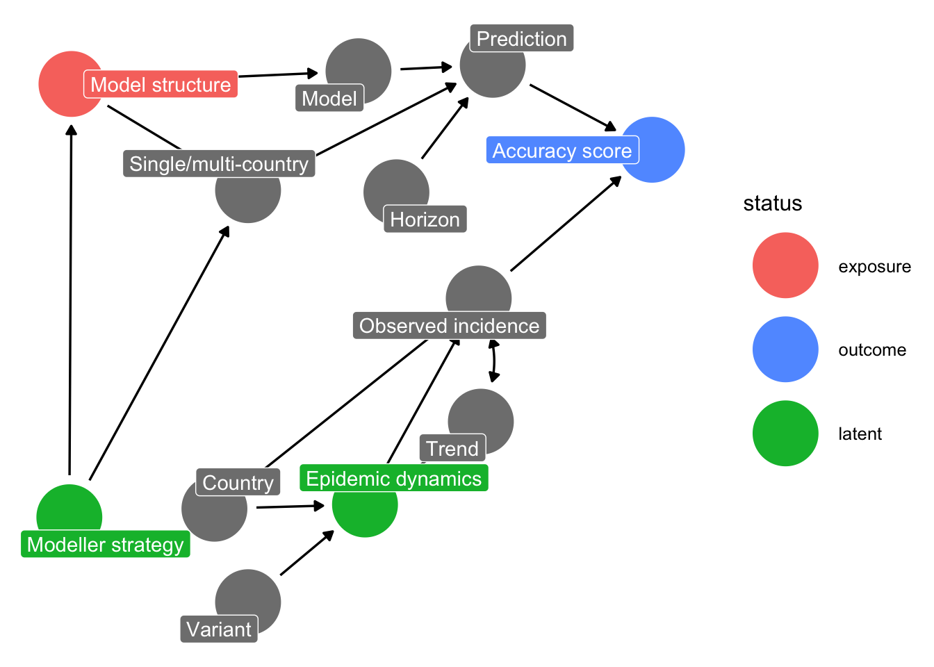
The epidemiological outcome enters the diagram as a confounder rather than simply a covariate. Forecasters chose which outcomes to submit predictions for, and that choice is associated with model structure, opening a backdoor path from structure to the score through modeller strategy. The outcome also changes the scale and reporting characteristics of the series being scored.
The joint model therefore adjusts for:
- Forecast target difficulty (which block backdoor paths from epidemic dynamics into the score), as:
EpiTarget,Trend,Horizon,Incidence,Location,VariantPhase
- Forecaster strategy, as:
CountryTargets,Model
Querying the diagram for a minimal sufficient adjustment set returns this exact set of covariates, for the direct effect of model structure on the score. It returns no valid adjustment set for the total effect: modeller strategy is unobserved and confounds model structure with the choice of geographic scope, so no set of measured covariates blocks that path. This is why we report a partial, direct association throughout rather than a total effect, and why residual confounding by unmeasured forecaster characteristics remains a limitation.
Adjustment gives the partial association between model structure and LWIS with these covariates held fixed at their observed values.
The joint model also fits an interaction between model structure and the epidemiological outcome, allowing a structure to predict one outcome relatively better than the other. This is effect modification rather than confounding. A causal diagram encodes conditional independence and not effect modification, so the interaction does not appear in the diagram and does not change the adjustment set.
Why no separate structure main effect
The crossed term s(Method, Epi_target, bs = "re") is an unconstrained zero-mean effect over all structure-by-outcome cells, so its average across outcomes is what a structure main effect would represent. With both terms in the model and both penalised, the division between them follows the relative variance estimates rather than the data: fitted together, mgcv gave the main effect 0.001 effective degrees of freedom against 4.9 for the crossed term, and dropping it left AIC, deviance explained and residuals unchanged. We therefore fit the crossed term alone and recover the pooled per-structure effect as a contrast averaging a structure’s two cells.
The same aliasing applies to the epidemiological outcome, whose main effect is the average of the crossed effects within an outcome. Here only one of the two terms is penalised, so the unpenalised fixed effect takes the component common to all structures and the crossed term keeps only departures from it. In the fitted model the crossed effects average to zero within each outcome to numerical precision, so the whole deaths-versus-cases difference sits in the fixed coefficient. This is emergent rather than imposed: the smooth retains all ten coefficients, so no centring constraint was applied. We did not treat the outcome as a random effect, which with two levels gives no basis for estimating a variance and would shrink a large, well-identified contrast toward zero.
Model fitting
We noted our outcome of LWIS had a strongly skewed PDF.
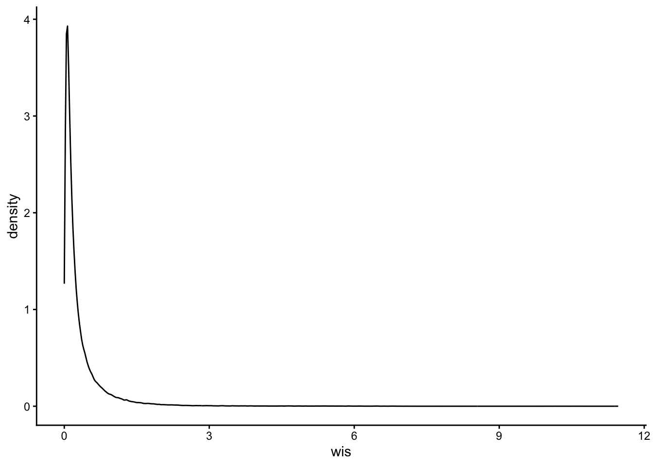
We therefore compared three error families on this specification, holding the formula and data fixed and varying only the family. The Gaussian family leaves the skew in the residuals rather than modelling it. The Gamma and Tweedie families both accommodate a right-skewed positive outcome, and fit this data almost identically. mgcv restricts the Tweedie power parameter to \(1 < p < 2\), and the estimate sits near the top of that range, so the data are asking for a variance function close to the Gamma (\(p = 2\)). The two fit this data almost identically, and both converge. We report the Tweedie fit because a Gamma has no support at zero: fitting it requires adding a constant to every score, which displaces the 553 forecasts that score exactly zero to a value set by the size of that constant.
The choice of family matters a great deal more the log scale than the natural scale. On the log scale, moving from Gaussian to Tweedie reduces residual skew from 5.8 to 0.6 and kurtosis from 77.6 to 10. On the natural scale, the WIS is heavily skewed, and the residual skew is essentially unchanged (1.84); there the change resolves the convergence failure rather than improving the distributional fit.
| Family | Deviance explained | AIC | Residual skew | Residual kurtosis |
|---|---|---|---|---|
| gaussian | 0.286 | 262955 | 5.85 | 77.6 |
| Gamma | 0.378 | -103418 | 0.52 | 9.5 |
| Tweedie(p=1.99) | 0.380 | -103165 | 0.58 | 9.3 |
A small share of forecasts (553, or 0.27%) score exactly zero: perfect predictions of zero-incidence targets, almost all deaths in the smallest countries. Gamma has no support at zero, so fitting it requires displacing these scores by a small constant. A Tweedie family with power parameter between 1 and 2 has a point mass at zero and admits them directly, so the primary model retains the exact zeros and adds no constant. Adding a constant of 1e-7 back to every score changes the fit very little (residual skew 0.58 against 0.57, deviance explained 0.380 against 0.382), so the choice is not consequential; we prefer the specification that represents the scores as they are.
We used the mgcv package v1.9-4 using R 4.5, with the formula:
wis ~ Epi_target + s(Method, Epi_target, bs = “re”) + s(CountryTargets, bs = “re”) + s(Incidence) + s(Trend, bs = “re”) + s(Location, bs = “re”) + s(VariantPhase, bs = “re”) + s(Horizon, by = Model, k = 3, bs = “sz”) + s(Model, bs = “re”)
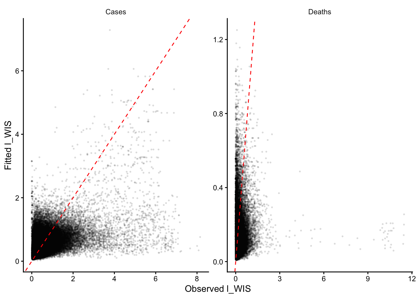
We assessed model fit visually plotting observed-versus-fitted values and inspecting residuals in Q-Q and histogram plots.

Results
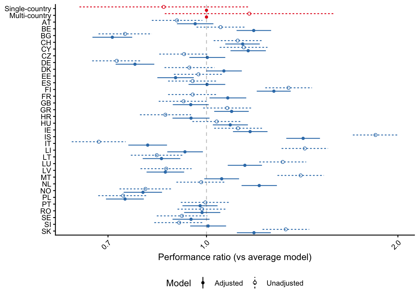
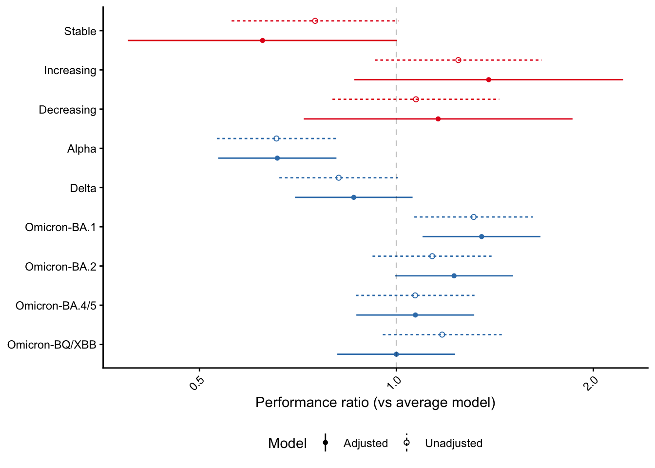
Effects are random effects for each level of a covariate, relative to a forecast at the average level of that covariate with all other terms held fixed. Negative raw effects, or ratios below 1, indicate better-than-average performance.
Partial effects across covariates
Partial effect on forecast performance of key covariates included in the fully adjusted model for additional covariates. Partial effects of individual model structure and individual model are presented in the main text.
- Geographic
- Epidemic state
Partial effects on the raw scale
The main-text figures and tables report exponentiated effects (multiplicative ratios of the expected LWIS relative to the average level of each factor). The table below gives the underlying raw partial effects from the fully adjusted model.
| Variable | Group | Partial effect (95% CI), log scale |
|---|---|---|
| CountryTargets | Multi-country | 0 (-0.005, 0.005) |
| Single-country | 0 (-0.005, 0.005) | |
| Epi_target | Deaths | -1.042 (-1.157, -0.926) |
| Location | AT | -0.117 (-0.211, -0.022) |
| BE | -0.064 (-0.158, 0.031) | |
| BG | -0.193 (-0.288, -0.098) | |
| CH | 0.011 (-0.083, 0.106) | |
| CY | 0.274 (0.179, 0.369) | |
| CZ | -0.11 (-0.204, -0.015) | |
| DE | -0.515 (-0.609, -0.42) | |
| DK | -0.175 (-0.269, -0.08) | |
| EE | 0.115 (0.02, 0.21) | |
| ES | -0.04 (-0.135, 0.054) | |
| FI | 0.319 (0.224, 0.414) | |
| FR | -0.254 (-0.349, -0.159) | |
| GB | -0.192 (-0.287, -0.097) | |
| GR | -0.001 (-0.096, 0.094) | |
| HR | -0.109 (-0.203, -0.014) | |
| HU | 0.035 (-0.059, 0.13) | |
| IE | 0.129 (0.035, 0.224) | |
| IS | 0.561 (0.465, 0.656) | |
| IT | -0.539 (-0.634, -0.444) | |
| LI | 0.57 (0.474, 0.665) | |
| LT | -0.118 (-0.212, -0.023) | |
| LU | 0.319 (0.224, 0.414) | |
| LV | 0.032 (-0.063, 0.126) | |
| MT | 0.417 (0.322, 0.512) | |
| NL | -0.078 (-0.173, 0.017) | |
| NO | -0.13 (-0.225, -0.036) | |
| PL | -0.365 (-0.459, -0.271) | |
| PT | -0.021 (-0.116, 0.074) | |
| RO | 0.026 (-0.069, 0.12) | |
| SE | -0.053 (-0.148, 0.041) | |
| SI | 0.002 (-0.092, 0.097) | |
| SK | 0.263 (0.168, 0.357) | |
| Method | Agent-based | -0.021 (-0.136, 0.095) |
| Judgement | -0.025 (-0.139, 0.089) | |
| Mechanistic | 0 (-0.099, 0.099) | |
| Semi-mechanistic | 0.053 (-0.053, 0.158) | |
| Statistical | -0.007 (-0.109, 0.095) | |
| Model | AMM-EpiInvert | -0.299 (-0.412, -0.187) |
| CovidMetrics-epiBATS | -0.128 (-0.276, 0.02) | |
| DSMPG-bayes | -0.48 (-0.617, -0.344) | |
| EuroCOVIDhub-baseline | 0.049 (-0.057, 0.156) | |
| FIAS_FZJ-Epi1Ger | 0.27 (0.142, 0.397) | |
| GoeWroc-BaseBayes | 0.555 (0.239, 0.871) | |
| HZI-AgeExtendedSEIR | -0.16 (-0.279, -0.04) | |
| ICM-agentModel | 0.128 (-0.029, 0.286) | |
| IEM_Health-CovidProject | -0.024 (-0.12, 0.073) | |
| ILM-EKF | 0.024 (-0.094, 0.142) | |
| ITWW-county_repro | 0.148 (0.019, 0.277) | |
| Imperial-DeCa | 0 (-0.452, 0.452) | |
| Imperial-RtI0 | 0 (-0.452, 0.452) | |
| Imperial-sbkp | 0 (-0.452, 0.452) | |
| JBUD-HMXK | 0.111 (0.009, 0.214) | |
| KITmetricslab-bivar_branching | 0.023 (-0.358, 0.405) | |
| Karlen-pypm | -0.154 (-0.252, -0.056) | |
| LANL-GrowthRate | -0.116 (-0.235, 0.003) | |
| LeipzigIMISE-SECIR | 0.068 (-0.219, 0.354) | |
| MIMUW-StochSEIR | 0.296 (0.12, 0.471) | |
| MIT_CovidAnalytics-DELPHI | 0.146 (0.03, 0.263) | |
| MOCOS-agent1 | -0.396 (-0.553, -0.24) | |
| MUNI-ARIMA | -0.1 (-0.207, 0.007) | |
| MUNI-LaggedRegARIMA | -0.167 (-0.296, -0.039) | |
| MUNI-VAR | 0.138 (0.024, 0.253) | |
| MUNI_DMS-SEIAR | -0.007 (-0.141, 0.128) | |
| PL_GRedlarski-DistrictsSum | -0.204 (-0.342, -0.065) | |
| RobertWalraven-ESG | 0.103 (-0.004, 0.21) | |
| SDSC_ISG-TrendModel | 0 (-0.452, 0.452) | |
| UB-BSLCoV | 0.073 (-0.098, 0.243) | |
| UC3M-EpiGraph | -0.007 (-0.331, 0.317) | |
| ULZF-SEIRC19SI | -0.336 (-0.467, -0.205) | |
| UMass-MechBayes | -0.144 (-0.243, -0.045) | |
| UMass-SemiMech | -0.016 (-0.137, 0.105) | |
| UNED-PreCoV2 | -0.041 (-0.204, 0.122) | |
| UNIPV-BayesINGARCHX | 0.445 (0.306, 0.584) | |
| USC-SIkJalpha | 0.132 (0.037, 0.228) | |
| UpgUmibUsi-MultiBayes | 0 (-0.452, 0.452) | |
| bisop-seirfilter | 0.013 (-0.222, 0.247) | |
| bisop-seirfilterlite | 0.097 (-0.024, 0.218) | |
| epiMOX-SUIHTER | -0.059 (-0.318, 0.201) | |
| epiforecasts-EpiExpert | -0.105 (-0.249, 0.039) | |
| epiforecasts-EpiExpert_Rt | -0.098 (-0.25, 0.054) | |
| epiforecasts-EpiExpert_direct | -0.127 (-0.28, 0.025) | |
| epiforecasts-EpiNow2 | 0.012 (-0.106, 0.129) | |
| epiforecasts-weeklygrowth | -0.187 (-0.296, -0.078) | |
| itwm-dSEIR | -0.043 (-0.161, 0.076) | |
| prolix-euclidean | 0.567 (0.441, 0.693) | |
| Trend | Decreasing | 0.048 (-0.201, 0.297) |
| Increasing | 0.192 (-0.057, 0.44) | |
| Stable | -0.24 (-0.488, 0.009) | |
| VariantPhase | Alpha | -0.193 (-0.327, -0.058) |
| Delta | -0.209 (-0.343, -0.074) | |
| Omicron-BA.1 | 0.196 (0.061, 0.33) | |
| Omicron-BA.2 | 0.106 (-0.029, 0.24) | |
| Omicron-BA.4/5 | 0.001 (-0.133, 0.135) | |
| Omicron-BQ/XBB | 0.099 (-0.036, 0.234) |
The model structure term is fitted as a single grouping factor crossing structure with epidemiological outcome, so its raw partial effects are one per structure-by-outcome cell. The main text reports these exponentiated, and reports a pooled effect per structure derived as a contrast averaging a structure’s two cells.
| Model structure | Cases | Deaths |
|---|---|---|
| Agent-based | 1.1 (0.96, 1.25) | 0.87 (0.76, 1) |
| Judgement | 0.96 (0.84, 1.09) | 0.99 (0.87, 1.13) |
| Mechanistic | 0.95 (0.85, 1.07) | 1.05 (0.94, 1.18) |
| Semi-mechanistic | 1.04 (0.92, 1.17) | 1.07 (0.95, 1.21) |
| Statistical | 0.96 (0.86, 1.08) | 1.02 (0.91, 1.15) |
| Model structure | Outcome | Partial effect (95% CI), log scale |
|---|---|---|
| Agent-based | Cases | 0.093 (-0.041, 0.227) |
| Deaths | -0.135 (-0.27, 0.001) | |
| Judgement | Cases | -0.044 (-0.174, 0.086) |
| Deaths | -0.006 (-0.137, 0.124) | |
| Mechanistic | Cases | -0.047 (-0.161, 0.068) |
| Deaths | 0.047 (-0.067, 0.162) | |
| Semi-mechanistic | Cases | 0.035 (-0.085, 0.155) |
| Deaths | 0.07 (-0.05, 0.191) | |
| Statistical | Cases | -0.037 (-0.154, 0.08) |
| Deaths | 0.023 (-0.094, 0.14) |
Model ranking before and after adjustment
Individual models can be ranked by their partial effect on the score, either from a univariate model containing only individual model identity, or from the fully adjusted model. The first ranks models by observed performance, and so by a combination of the method used and the difficulty of the targets each model chose to forecast. The second ranks them by performance after the target-related covariates are held fixed. The comparison is reported in the main text; the table below gives the models that move furthest between the two.
| Model | Unadjusted rank | Adjusted rank | Rank change |
|---|---|---|---|
| Statistical 11 | 43 | 6 | 37 |
| Statistical 10 | 40 | 4 | 36 |
| Mechanistic 15 | 35 | 5 | 30 |
| Semi-mechanistic 1 | 1 | 28 | -27 |
| Agent-based 3 | 46 | 23 | 23 |
| Semi-mechanistic 2 | 2 | 24 | -22 |
| Semi-mechanistic 3 | 4 | 26 | -22 |
| Mechanistic 4 | 12 | 34 | -22 |
| Statistical 6 | 32 | 11 | 21 |
| Mechanistic 9 | 21 | 42 | -21 |
Sensitivity analyses
Data processing
Population normalisation
We scored forecasts and observations normalised by country population per 100,000. We also scored against the raw total incident weekly count per target. This had near-zero impact on model fitting or results on the log-transformed scores. Difference in median WIS (across all targets):
| Target | Scale | Raw count | Per 100k |
|---|---|---|---|
| Cases | log | 0.292 | 0.278 |
| Cases | natural | 2426 | 34.4 |
| Deaths | log | 0.239 | 0.093 |
| Deaths | natural | 14.7 | 0.199 |
Natural scale WIS
We present results from scoring forecast error on the natural scale (difference between observation and prediction in count of case or death incidence), from which the WIS is then calculated and the analysis repeated.
| Models (%) | Models (%) | Models (%) | Participation (%) | |
|---|---|---|---|---|
| Overall | 43 (100%) | 39 (100%) | 48 (100%) | 3% |
| Method | ||||
| Semi-mechanistic | 9 (20.9%) | 10 (25.6%) | 12 (25%) | 4% |
| Statistical | 12 (27.9%) | 8 (20.5%) | 13 (27.1%) | 7% |
| Mechanistic | 16 (37.2%) | 16 (41%) | 17 (35.4%) | 3% |
| Agent-based | 3 (7%) | 2 (5.1%) | 3 (6.2%) | 3% |
| Judgement | 3 (7%) | 3 (7.7%) | 3 (6.2%) | 3% |
Model specification
We tried several alternative model specifications.
Covariate selection
| Domain | Variable | Model version | Impact |
|---|---|---|---|
| Forecast target | |||
EpiTarget |
V2* | None | |
VariantPhase |
V2* | Some | |
Trend |
All | Untested | |
Horizon |
All | Untested | |
Incidence |
All | Untested | |
Location |
All | Untested | |
| Forecaster strategy | |||
CountryTargets |
All | Untested | |
Model |
All | Untested | |
| Outcome | Method |
All |
* Covariates included in V2 were added based on reviewer feedback.
Error family and link
We first used a Gaussian distribution with a log link. Because LWIS is strongly right-skewed, this left high residual skewness (5.8) and kurtosis (77.6). We avoid using additional data transformations (e.g. an additional log transform) on the outcome (LWIS) as this would violate propriety of the score. We instead addressed the skew through the error family, comparing Gaussian, Gamma and Tweedie families as reported under Model fitting above, and adopting the Tweedie family for the reported analysis.
The fitted relationships and partial effects remained stable across parameterisations.
Structure by outcome under a Gaussian family
The structure-by-outcome effects are sensitive to the error family, in magnitude throughout and in direction for two of the five structures. The table below refits the same specification with a Gaussian family and log link, alongside the primary Tweedie fit. The case-versus-death contrast keeps its sign under the Gaussian family for judgement, mechanistic and statistical models. It does not for agent-based models, where the separation vanishes, or for semi-mechanistic models, where it reverses; in both the Gaussian contrast is close to zero. The Gaussian fit is dominated by the largest scores, which fall disproportionately among case forecasts, so it weights precisely the observations the Tweedie family is chosen to accommodate. Including or excluding the Hub baseline model makes no material difference to these estimates. We report the Tweedie fit throughout; the size of any single structure-by-outcome contrast should be read with this sensitivity in mind.
| Model structure | Outcome | Tweedie | Gaussian |
|---|---|---|---|
| Agent-based | Cases | 1.10 | 0.99 |
| Deaths | 0.87 | 1.00 | |
| Judgement | Cases | 0.96 | 0.97 |
| Deaths | 0.99 | 1.03 | |
| Mechanistic | Cases | 0.95 | 0.98 |
| Deaths | 1.05 | 1.00 | |
| Semi-mechanistic | Cases | 1.04 | 1.06 |
| Deaths | 1.07 | 0.97 | |
| Statistical | Cases | 0.96 | 1.00 |
| Deaths | 1.02 | 1.01 |