Supplementary material
Methods
Source data and code
Forecast and observed data were sourced from the European COVID-19 Forecast Hub, available to view at https://covid19forecasthub.eu/ . All Hub data are now archived at:
- Github: https://github.com/european-modelling-hubs/covid19-forecast-hub-europe_archive
- Zenodo with DOI: https://doi.org/10.5281/zenodo.13986751
Data for this work were downloaded on 30th May 2023. These data are available in the Github repository for this paper at: https://github.com/epiforecasts/eval-by-method/tree/main/data
The codebase for this paper is publicly available at:
- Github: https://github.com/epiforecasts/eval-by-method
- Zenodo with DOI: https://doi.org/10.5281/zenodo.14903162
Comments and code contributions are welcome - please use Github Issues.
Please cite code using:
- Katharine Sherratt & Sebastian Funk. (2025). epiforecasts/eval-by-method: Zenodo. https://doi.org/10.5281/zenodo.14903162
Study participation
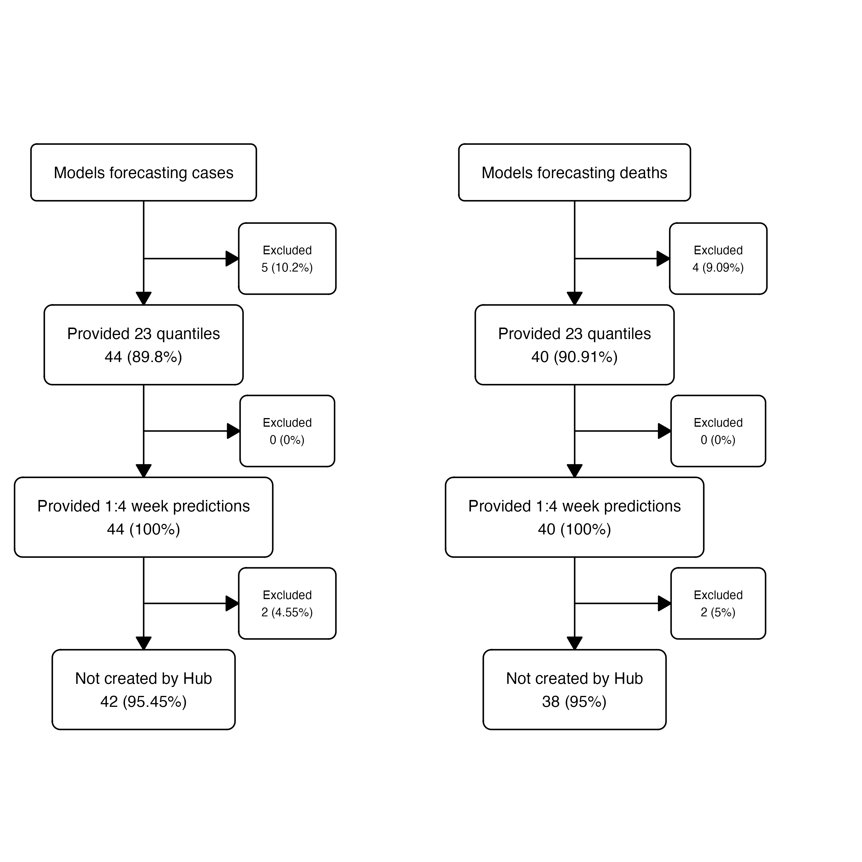
Forecasting teams were recruited to the European Covid-19 Forecast Hub using existing networks and ECDC publicity. Any forecaster was eligible to participate, and there were no selection criteria. All participation was voluntary and unrenumerated. Forecasters contributed a standard set of metadata describing their team and model, and uploaded forecasts weekly. Forecasters were optionally able to express uncertainty by reporting a distribution of up to 23 probabilistic quantiles for each prediction. Forecasts were validated against minimal formatting requirements for quantile intervals and that values were positive integers.
For this study, we collected all forecasts from between 8 March 2021 to 10 March 2023. We excluded forecasts of hospitalisations, which experienced multiple changes in source data during the study period. We excluded forecasts that did not report the full set of 23 quantiles, in order to ensure fair comparison among probabilistic model results. We also excluded baseline and ensemble models created by the Hub team.
Characteristics of contributing models:
| Model | Method | Country Targets | Case forecasts | Death forecasts |
|---|---|---|---|---|
| AMM-EpiInvert | Statistical | Multi-country | 2,788 | |
| CovidMetrics-epiBATS | Statistical | Single-country | 343 | |
| DSMPG-bayes | Semi-mechanistic | Multi-country | 760 | |
| EuroCOVIDhub-baseline | Statistical | Multi-country | 13,082 | 13,040 |
| FIAS_FZJ-Epi1Ger | Mechanistic | Single-country | 264 | 264 |
| GoeWroc-BaseBayes | Semi-mechanistic | Single-country | 12 | |
| HZI-AgeExtendedSEIR | Mechanistic | Single-country | 382 | 382 |
| ICM-agentModel | Agent-based | Single-country | 334 | 334 |
| IEM_Health-CovidProject | Mechanistic | Multi-country | 7,710 | 7,708 |
| ILM-EKF | Semi-mechanistic | Multi-country | 11,998 | 11,961 |
| ITWW-county_repro | Semi-mechanistic | Multi-country | 650 | 600 |
| Imperial-DeCa | Semi-mechanistic | Multi-country | 571 | |
| Imperial-RtI0 | Semi-mechanistic | Multi-country | 571 | |
| Imperial-sbkp | Semi-mechanistic | Multi-country | 571 | |
| JBUD-HMXK | Mechanistic | Multi-country | 1,324 | 1,324 |
| KITmetricslab-bivar_branching | Statistical | Single-country | 8 | |
| Karlen-pypm | Mechanistic | Multi-country | 3,208 | 3,186 |
| LANL-GrowthRate | Semi-mechanistic | Multi-country | 3,692 | 3,696 |
| LeipzigIMISE-SECIR | Mechanistic | Single-country | 16 | 16 |
| MIMUW-StochSEIR | Mechanistic | Single-country | 76 | 76 |
| MIT_CovidAnalytics-DELPHI | Mechanistic | Multi-country | 348 | 500 |
| MOCOS-agent1 | Agent-based | Single-country | 386 | 386 |
| MUNI-ARIMA | Statistical | Multi-country | 10,979 | 11,314 |
| MUNI-LaggedRegARIMA | Statistical | Multi-country | 736 | |
| MUNI-VAR | Statistical | Multi-country | 976 | 976 |
| MUNI_DMS-SEIAR | Mechanistic | Single-country | 224 | 200 |
| PL_GRedlarski-DistrictsSum | Mechanistic | Single-country | 378 | |
| RobertWalraven-ESG | Statistical | Multi-country | 9,190 | 10,465 |
| SDSC_ISG-TrendModel | Statistical | Multi-country | 1,756 | 1,744 |
| UB-BSLCoV | Statistical | Single-country | 96 | 96 |
| UC3M-EpiGraph | Agent-based | Single-country | 94 | |
| ULZF-SEIRC19SI | Mechanistic | Single-country | 249 | 249 |
| UMass-MechBayes | Mechanistic | Multi-country | 5,948 | |
| UMass-SemiMech | Semi-mechanistic | Multi-country | 1,888 | 1,904 |
| UNED-PreCoV2 | Statistical | Single-country | 147 | 147 |
| UNIPV-BayesINGARCHX | Statistical | Multi-country | 426 | |
| USC-SIkJalpha | Mechanistic | Multi-country | 12,900 | 12,688 |
| UpgUmibUsi-MultiBayes | Semi-mechanistic | Single-country | 99 | 99 |
| bisop-seirfilter | Mechanistic | Single-country | 32 | 32 |
| bisop-seirfilterlite | Mechanistic | Multi-country | 336 | 336 |
| epiMOX-SUIHTER | Mechanistic | Single-country | 134 | 134 |
| epiforecasts-EpiExpert | Judgement | Multi-country | 945 | 948 |
| epiforecasts-EpiExpert_Rt | Judgement | Multi-country | 404 | 404 |
| epiforecasts-EpiExpert_direct | Judgement | Multi-country | 394 | 392 |
| epiforecasts-EpiNow2 | Semi-mechanistic | Multi-country | 8,843 | 7,721 |
| epiforecasts-weeklygrowth | Statistical | Multi-country | 5,971 | |
| itwm-dSEIR | Mechanistic | Single-country | 406 | 406 |
| prolix-euclidean | Semi-mechanistic | Multi-country | 800 | 800 |
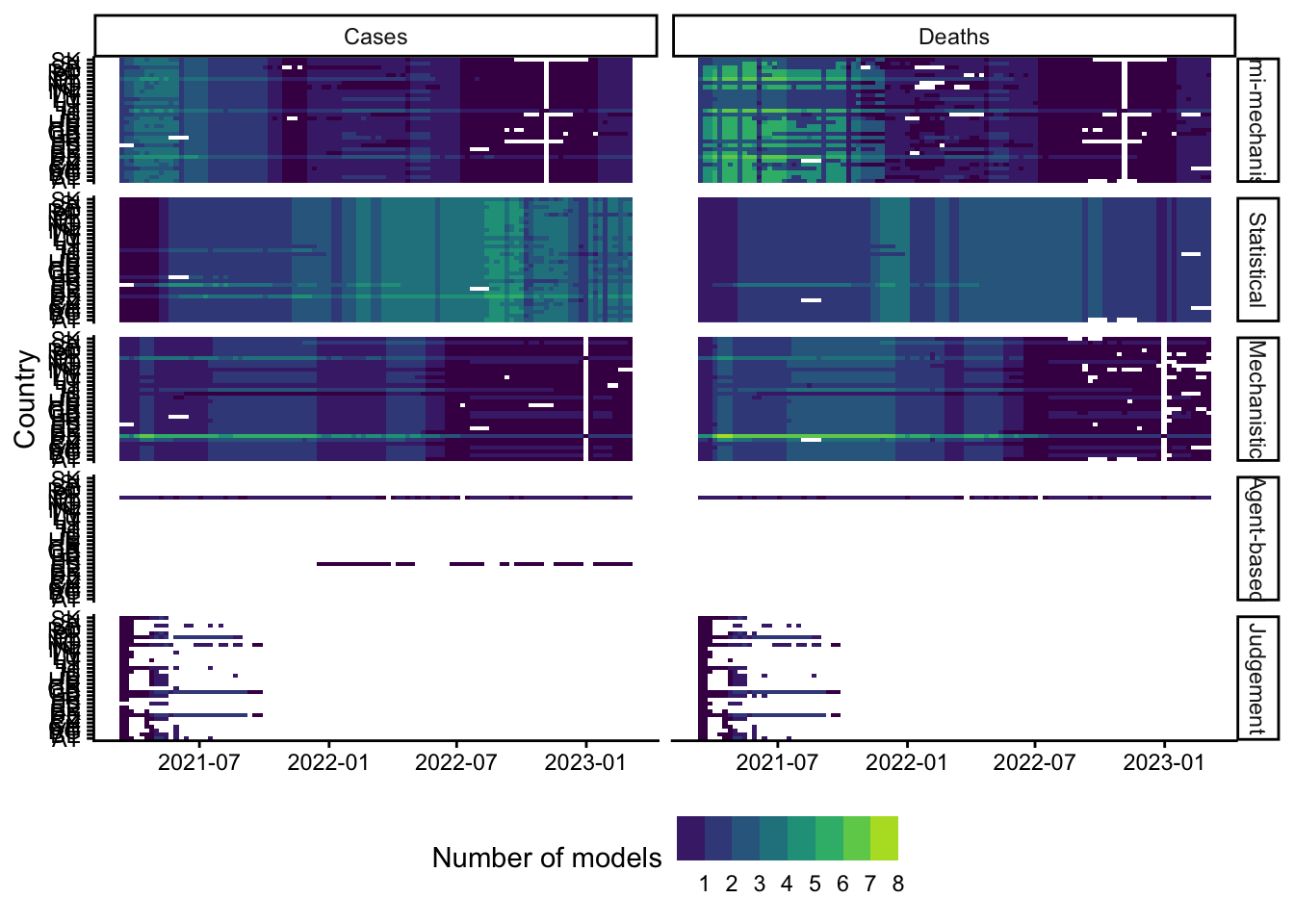
Number of models participating in forecasting 1-week ahead case incidence for each country over the study period.
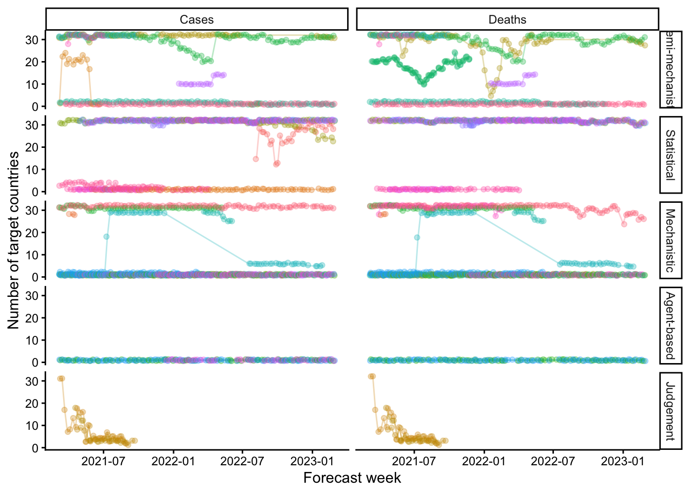
We explored how models selected geographic targets over time. Forecasters both added and removed targets among the set for which they forecast each week. This figure shows number of targets submitted by each model at the 1-week ahead horizon. We noted the same variation for 2-4 week forecasts.
Model structure classification
Human raters classified models according to methodological structures.
| Model | Final classification | Agreement | Total raters | Semi-mechanistic | Mechanistic | Agent-based | Statistical | Judgement | Other | Machine Learning |
|---|---|---|---|---|---|---|---|---|---|---|
| AMM-EpiInvert | Statistical | FALSE | 3 | 0 | 0 | 0 | 2 | 0 | 1 | 0 |
| DSMPG-bayes | Semi-mechanistic | FALSE | 3 | 2 | 0 | 0 | 1 | 0 | 0 | 0 |
| ILM-EKF | Semi-mechanistic | FALSE | 3 | 2 | 0 | 0 | 1 | 0 | 0 | 0 |
| ITWW-county_repro | Semi-mechanistic | FALSE | 3 | 2 | 0 | 0 | 1 | 0 | 0 | 0 |
| Imperial-DeCa | Semi-mechanistic | FALSE | 3 | 2 | 0 | 0 | 1 | 0 | 0 | 0 |
| Imperial-RtI0 | Semi-mechanistic | FALSE | 3 | 2 | 0 | 0 | 1 | 0 | 0 | 0 |
| Imperial-sbkp | Semi-mechanistic | FALSE | 3 | 2 | 0 | 0 | 1 | 0 | 0 | 0 |
| KITmetricslab-bivar_branching | Statistical | FALSE | 3 | 1 | 0 | 0 | 2 | 0 | 0 | 0 |
| Karlen-pypm | Mechanistic | FALSE | 3 | 0 | 2 | 0 | 1 | 0 | 0 | 0 |
| LANL-GrowthRate | Semi-mechanistic | FALSE | 3 | 2 | 0 | 0 | 1 | 0 | 0 | 0 |
| SDSC_ISG-TrendModel | Statistical | FALSE | 3 | 0 | 0 | 0 | 2 | 0 | 1 | 0 |
| UMass-SemiMech | Semi-mechanistic | FALSE | 4 | 3 | 1 | 0 | 0 | 0 | 0 | 0 |
| USC-SIkJalpha | Mechanistic | FALSE | 4 | 1 | 3 | 0 | 0 | 0 | 0 | 0 |
| UpgUmibUsi-MultiBayes | Semi-mechanistic | FALSE | 3 | 2 | 0 | 0 | 1 | 0 | 0 | 0 |
| bisop-seirfilter | Mechanistic | FALSE | 4 | 1 | 3 | 0 | 0 | 0 | 0 | 0 |
| bisop-seirfilterlite | Mechanistic | FALSE | 4 | 1 | 3 | 0 | 0 | 0 | 0 | 0 |
| prolix-euclidean | Semi-mechanistic | FALSE | 4 | 3 | 0 | 0 | 0 | 0 | 1 | 0 |
| CovidMetrics-epiBATS | Statistical | TRUE | 3 | 0 | 0 | 0 | 3 | 0 | 0 | 0 |
| EuroCOVIDhub-baseline | Statistical | TRUE | 4 | 0 | 0 | 0 | 4 | 0 | 0 | 0 |
| FIAS_FZJ-Epi1Ger | Mechanistic | TRUE | 3 | 0 | 3 | 0 | 0 | 0 | 0 | 0 |
| GoeWroc-BaseBayes | Semi-mechanistic | TRUE | 3 | 3 | 0 | 0 | 0 | 0 | 0 | 0 |
| HZI-AgeExtendedSEIR | Mechanistic | TRUE | 3 | 0 | 3 | 0 | 0 | 0 | 0 | 0 |
| ICM-agentModel | Agent-based | TRUE | 3 | 0 | 0 | 3 | 0 | 0 | 0 | 0 |
| IEM_Health-CovidProject | Mechanistic | TRUE | 4 | 0 | 4 | 0 | 0 | 0 | 0 | 0 |
| JBUD-HMXK | Mechanistic | TRUE | 3 | 0 | 3 | 0 | 0 | 0 | 0 | 0 |
| LeipzigIMISE-SECIR | Mechanistic | TRUE | 3 | 0 | 3 | 0 | 0 | 0 | 0 | 0 |
| MIMUW-StochSEIR | Mechanistic | TRUE | 3 | 0 | 3 | 0 | 0 | 0 | 0 | 0 |
| MIT_CovidAnalytics-DELPHI | Mechanistic | TRUE | 3 | 0 | 3 | 0 | 0 | 0 | 0 | 0 |
| MOCOS-agent1 | Agent-based | TRUE | 3 | 0 | 0 | 3 | 0 | 0 | 0 | 0 |
| MUNI-ARIMA | Statistical | TRUE | 3 | 0 | 0 | 0 | 3 | 0 | 0 | 0 |
| MUNI-LaggedRegARIMA | Statistical | TRUE | 3 | 0 | 0 | 0 | 3 | 0 | 0 | 0 |
| MUNI-VAR | Statistical | TRUE | 3 | 0 | 0 | 0 | 3 | 0 | 0 | 0 |
| MUNI_DMS-SEIAR | Mechanistic | TRUE | 3 | 0 | 3 | 0 | 0 | 0 | 0 | 0 |
| PL_GRedlarski-DistrictsSum | Mechanistic | TRUE | 3 | 0 | 3 | 0 | 0 | 0 | 0 | 0 |
| RobertWalraven-ESG | Statistical | TRUE | 3 | 0 | 0 | 0 | 3 | 0 | 0 | 0 |
| UB-BSLCoV | Statistical | TRUE | 3 | 0 | 0 | 0 | 3 | 0 | 0 | 0 |
| UC3M-EpiGraph | Agent-based | TRUE | 3 | 0 | 0 | 3 | 0 | 0 | 0 | 0 |
| ULZF-SEIRC19SI | Mechanistic | TRUE | 3 | 0 | 3 | 0 | 0 | 0 | 0 | 0 |
| UMass-MechBayes | Mechanistic | TRUE | 3 | 0 | 3 | 0 | 0 | 0 | 0 | 0 |
| UNED-PreCoV2 | Statistical | TRUE | 3 | 0 | 0 | 0 | 3 | 0 | 0 | 0 |
| UNIPV-BayesINGARCHX | Statistical | TRUE | 3 | 0 | 0 | 0 | 3 | 0 | 0 | 0 |
| epiMOX-SUIHTER | Mechanistic | TRUE | 3 | 0 | 3 | 0 | 0 | 0 | 0 | 0 |
| epiforecasts-EpiExpert | Judgement | TRUE | 3 | 0 | 0 | 0 | 0 | 3 | 0 | 0 |
| epiforecasts-EpiExpert_Rt | Judgement | TRUE | 3 | 0 | 0 | 0 | 0 | 3 | 0 | 0 |
| epiforecasts-EpiExpert_direct | Judgement | TRUE | 3 | 0 | 0 | 0 | 0 | 3 | 0 | 0 |
| epiforecasts-EpiNow2 | Semi-mechanistic | TRUE | 3 | 3 | 0 | 0 | 0 | 0 | 0 | 0 |
| epiforecasts-weeklygrowth | Statistical | TRUE | 2 | 0 | 0 | 0 | 2 | 0 | 0 | 0 |
| itwm-dSEIR | Mechanistic | TRUE | 3 | 0 | 3 | 0 | 0 | 0 | 0 | 0 |
Epidemic trend identification
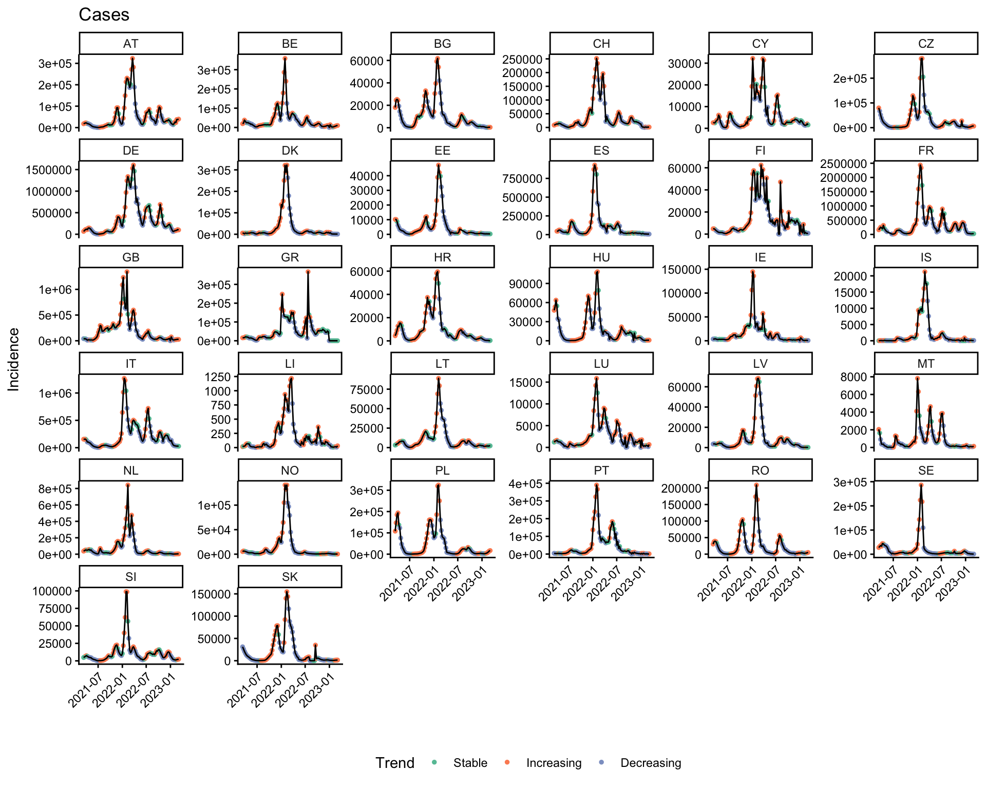
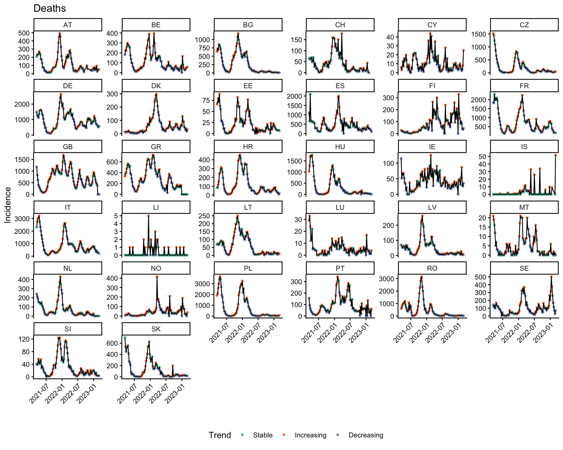
We categorised each week as “Stable”, “Decreasing”, or “Increasing”, based on the difference over a three-week moving average of incidence (with a change of +/-5% as “Stable”).
Variant phase identification
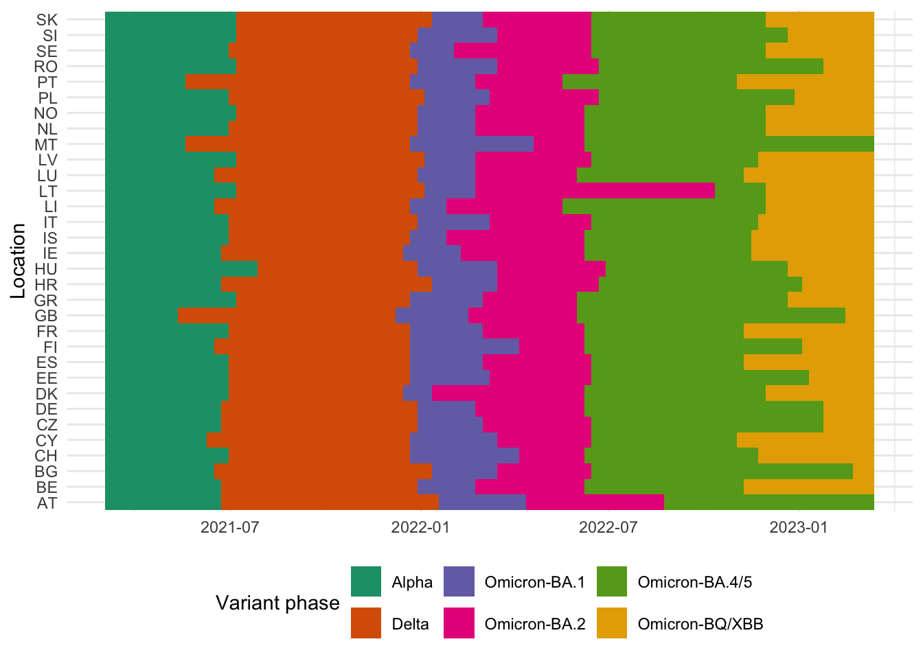
Genomic surveillance data were obtained from three sources: ECDC (covering 30 European countries), UKHSA (Great Britain), and the Swiss Federal Office of Public Health (Switzerland). Variant lineages were mapped to six named phases in expected chronological order: Alpha, Delta, Omicron-BA.1, Omicron-BA.2, Omicron-BA.4/5, and Omicron-BQ/XBB. For each country, we identified the first week in which each named variant exceeded 50% of sequenced samples. We enforced chronological ordering by removing any out-of-sequence phases, then expanded phase assignments to all weeks by filling forward and backward from observed transition dates. This per-location approach accounts for the fact that variant dominance dates differed substantially across European countries. Where genomic surveillance data were too sparse to identify a transition (Hungary), we supplemented with epidemiological reports to set the Alpha-to-Delta transition date.
Model building
To illustrate our approach to forecast evaluation, we show the assumptions underlying our adjustment strategy in a causal diagram. We emphasise that this work is exploratory rather than inferential, and we suggest substantial further work is needed to support inferential approaches to forecast evaluation.
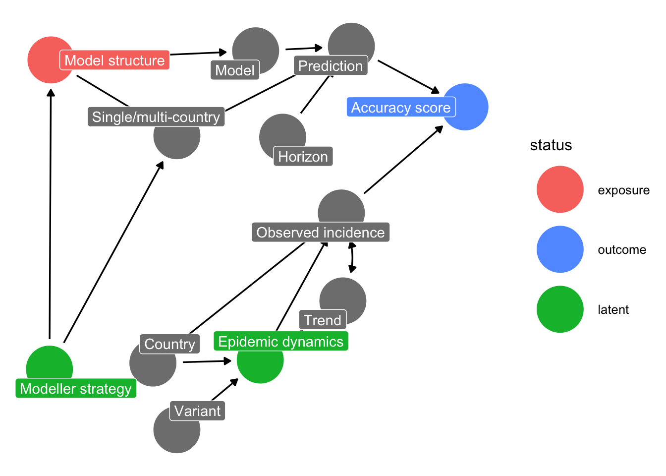
The joint model fitted in the main analysis adjusts for target-difficulty variables (Trend, Horizon, Incidence, Location, VariantPhase), which block backdoor paths from epidemic dynamics into the score, and additionally conditions on target strategy (CountryTargets) and individual model identity (Model). Adjustment gives the partial association between Method and log-WIS with these covariates held fixed at their observed values.
We used the following model formula with the mgcv package in R 4.1.
wis ~ Epi_target + s(Method, bs = “re”) + s(CountryTargets, bs = “re”) + s(Incidence) + s(Trend, bs = “re”) + s(Location, bs = “re”) + s(VariantPhase, bs = “re”) + s(Horizon, by = Model, k = 3, bs = “sz”) + s(Model, bs = “re”)
Results
Model diagnostics
Diagnostic plots (QQ, residuals vs linear predictor, histogram of residuals, and observed vs fitted) for the single combined model fitted jointly across both epidemiological targets.

The primary model uses a Gaussian family with a log link applied to the (untransformed) weighted interval score. This models the score multiplicatively but assumes additive, constant-variance Gaussian residuals on the raw score scale. Because the WIS is strongly right-skewed, the observation-level residuals retain a heavy upper tail (residual skewness ≈ 5.5, excess kurtosis well above the Gaussian reference), visible in the QQ plot above. The fitted relationships and partial effects are nonetheless stable: a reparameterisation that instead models the log-transformed score directly (below) substantially improves the residual distribution without materially changing the estimated effects.
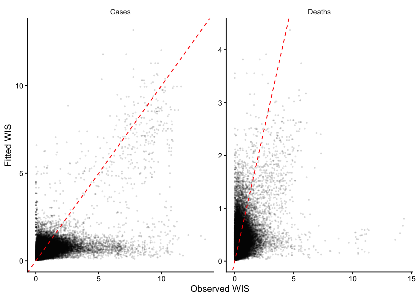
Observed versus fitted WIS for the primary model is shown below; points concentrate along the identity line, with the dispersion in the upper tail reflecting the residual skewness noted above.
Temporal autocorrelation
#TODO: This section is under substantial review
The model carries no temporal correlation structure, so it treats forecast scores as conditionally independent given the random effects. Scores are, however, a weekly repeated-measures series (by forecast date) at horizons 1–4, so we checked for residual autocorrelation that could bias the standard errors on the focal effects. We quantify autocorrelation on the log-response residuals (the near-symmetric gaussian(identity) reparameterisation; the primary log-link residuals are too skewed for a meaningful autocorrelation function), and compare against the raw log(WIS) series on the same scale. Each series is one weekly sequence at a fixed model–location–horizon–target combination (3,353 series with ≥ 10 weekly points).
The same within-origin dependence is visible directly in the residuals: across a sample of forecast origins (each black line is one model–location–date, traced over its four horizons), the residuals move together rather than crossing at random, so a forecast that is mis-scored at one horizon tends to be mis-scored in the same direction at the others.
Because the four horizons on a given origin date share the same observed data and target trajectory, we note this moderate-to-strong correlated dependence within forecast origins. The reported standard errors are therefore likely too narrow (a lower bound on the true uncertainty). An origin-level random effect would absorb this correlation, but because trend, variant, incidence and location are constant within an origin, such a term is collinear with them and cannot be estimated alongside them. We flag this as a limitation rather than refitting: the focal effects of model structure and geographic scope are identified across many origins rather than within them, whereas the between-origin covariates most exposed to the understated precision — epidemic trend and variant phase — are reported as secondary descriptive estimates and not the basis of our conclusions. The unchanged conclusions under the log-response reparameterisation (below) give no indication that this dependence alters the substantive findings.
Partial effects across covariates
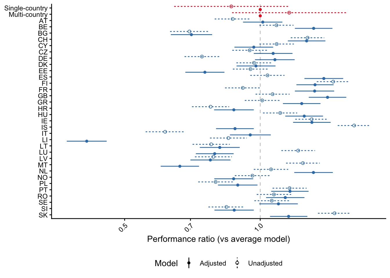
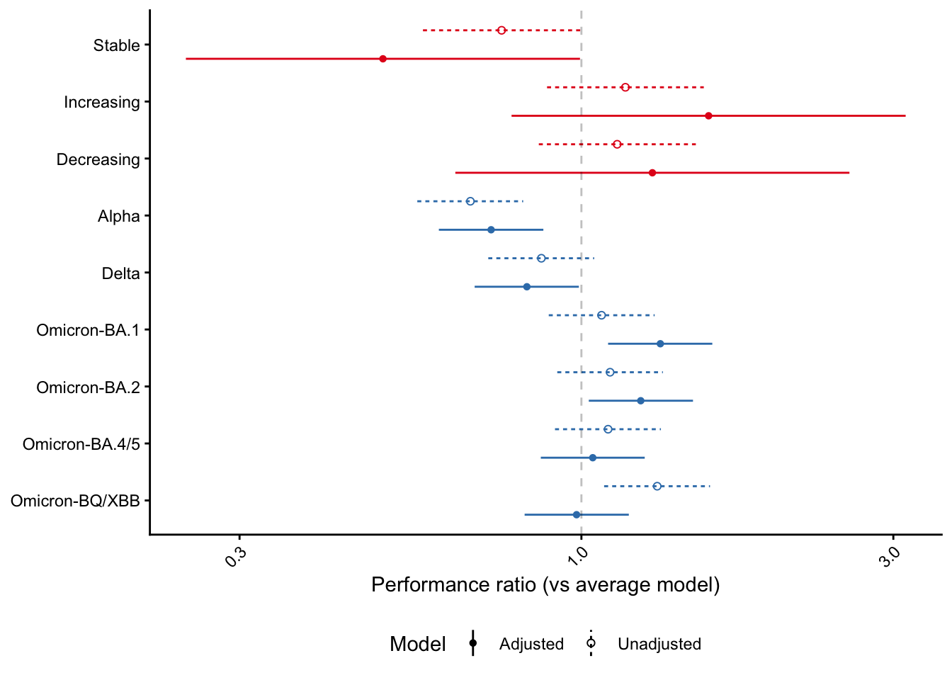
Partial effect on forecast performance of key covariates included in the fully adjusted model for (A) spatial and (B) temporal covariates. Partial effects of individual model structure and individual model are presented in main text. The full model included covariates for: model structure, individual model, number of countries targeted by a given model, the specific country target, the epidemic trend in the 3 weeks around the target, and the dominant variant at the time of the target.
- Spatial covariates
- Temporal covariates
- Raw partial effects on the log scale
The main-text figures and tables report exponentiated effects (multiplicative ratios relative to the grand-mean WIS). For reference and reproducibility, the table below gives the underlying raw partial effects on the log-WIS scale, with 95% confidence intervals, from the fully adjusted joint model. Negative values indicate better-than-average performance; effects are deviations from the grand mean under a sum-to-zero constraint.
| Variable | Group | Partial effect (95% CI), log scale |
|---|---|---|
| CountryTargets | Multi-country | 0 (-0.002, 0.002) |
| Single-country | 0 (-0.002, 0.002) | |
| Epi_target | Deaths | -1.316 (-1.334, -1.298) |
| Location | AT | 0.013 (-0.088, 0.113) |
| BE | 0.273 (0.177, 0.369) | |
| BG | -0.352 (-0.457, -0.246) | |
| CH | 0.237 (0.141, 0.333) | |
| CY | -0.033 (-0.132, 0.066) | |
| CZ | 0.066 (-0.033, 0.165) | |
| DE | 0.075 (-0.027, 0.176) | |
| DK | -0.022 (-0.121, 0.078) | |
| EE | -0.283 (-0.383, -0.183) | |
| ES | 0.325 (0.226, 0.424) | |
| FI | 0.28 (0.185, 0.375) | |
| FR | 0.278 (0.177, 0.378) | |
| GB | 0.344 (0.248, 0.44) | |
| GR | 0.212 (0.116, 0.308) | |
| HR | -0.135 (-0.236, -0.033) | |
| HU | 0.225 (0.128, 0.321) | |
| IE | 0.264 (0.168, 0.36) | |
| IS | -0.129 (-0.226, -0.033) | |
| IT | -0.051 (-0.155, 0.054) | |
| LI | -0.887 (-0.989, -0.785) | |
| LT | -0.207 (-0.309, -0.105) | |
| LU | -0.233 (-0.329, -0.136) | |
| LV | -0.255 (-0.357, -0.152) | |
| MT | -0.411 (-0.509, -0.313) | |
| NL | 0.272 (0.174, 0.371) | |
| NO | -0.136 (-0.235, -0.036) | |
| PL | -0.115 (-0.216, -0.014) | |
| PT | 0.152 (0.056, 0.247) | |
| RO | 0.128 (0.03, 0.226) | |
| SE | 0.093 (-0.005, 0.192) | |
| SI | -0.133 (-0.234, -0.033) | |
| SK | 0.145 (0.05, 0.241) | |
| Method | Agent-based | 0 (-0.002, 0.002) |
| Judgement | 0 (-0.002, 0.002) | |
| Mechanistic | 0 (-0.002, 0.002) | |
| Semi-mechanistic | 0 (-0.002, 0.002) | |
| Statistical | 0 (-0.002, 0.002) | |
| Model | AMM-EpiInvert | 0.14 (0.062, 0.217) |
| CovidMetrics-epiBATS | -0.094 (-0.293, 0.105) | |
| DSMPG-bayes | -0.348 (-0.54, -0.156) | |
| FIAS_FZJ-Epi1Ger | -0.017 (-0.209, 0.175) | |
| GoeWroc-BaseBayes | 0.165 (-0.239, 0.569) | |
| HZI-AgeExtendedSEIR | -0.098 (-0.281, 0.085) | |
| ICM-agentModel | 0.163 (0.017, 0.309) | |
| IEM_Health-CovidProject | -0.175 (-0.255, -0.094) | |
| ILM-EKF | 0.08 (0.005, 0.155) | |
| ITWW-county_repro | -0.088 (-0.232, 0.056) | |
| Imperial-DeCa | 0 (-0.426, 0.426) | |
| Imperial-RtI0 | 0 (-0.426, 0.426) | |
| Imperial-sbkp | 0 (-0.426, 0.426) | |
| JBUD-HMXK | 0.015 (-0.073, 0.103) | |
| KITmetricslab-bivar_branching | -0.058 (-0.452, 0.336) | |
| Karlen-pypm | -0.07 (-0.153, 0.012) | |
| LANL-GrowthRate | 0.012 (-0.071, 0.095) | |
| LeipzigIMISE-SECIR | -0.045 (-0.435, 0.346) | |
| MIMUW-StochSEIR | 0.164 (-0.103, 0.431) | |
| MIT_CovidAnalytics-DELPHI | 0.297 (0.143, 0.451) | |
| MOCOS-agent1 | -0.367 (-0.562, -0.171) | |
| MUNI-ARIMA | -0.057 (-0.133, 0.019) | |
| MUNI-LaggedRegARIMA | -0.316 (-0.512, -0.119) | |
| MUNI-VAR | 0.21 (0.101, 0.32) | |
| MUNI_DMS-SEIAR | -0.014 (-0.183, 0.156) | |
| PL_GRedlarski-DistrictsSum | -0.318 (-0.526, -0.109) | |
| RobertWalraven-ESG | 0.157 (0.081, 0.233) | |
| SDSC_ISG-TrendModel | 0 (-0.426, 0.426) | |
| UB-BSLCoV | -0.031 (-0.274, 0.212) | |
| UC3M-EpiGraph | -0.071 (-0.408, 0.265) | |
| ULZF-SEIRC19SI | -0.263 (-0.453, -0.072) | |
| UMass-MechBayes | -0.12 (-0.214, -0.027) | |
| UMass-SemiMech | 0.111 (0.023, 0.199) | |
| UNED-PreCoV2 | 0.025 (-0.206, 0.256) | |
| UNIPV-BayesINGARCHX | 0.195 (0.029, 0.362) | |
| USC-SIkJalpha | 0.166 (0.091, 0.241) | |
| UpgUmibUsi-MultiBayes | 0 (-0.426, 0.426) | |
| bisop-seirfilter | 0.018 (-0.337, 0.374) | |
| bisop-seirfilterlite | 0.083 (-0.091, 0.257) | |
| epiMOX-SUIHTER | 0.003 (-0.389, 0.396) | |
| epiforecasts-EpiExpert | -0.097 (-0.22, 0.026) | |
| epiforecasts-EpiExpert_Rt | -0.09 (-0.251, 0.07) | |
| epiforecasts-EpiExpert_direct | -0.076 (-0.225, 0.073) | |
| epiforecasts-EpiNow2 | 0.084 (0.007, 0.161) | |
| epiforecasts-weeklygrowth | -0.082 (-0.16, -0.004) | |
| itwm-dSEIR | 0.074 (-0.099, 0.247) | |
| prolix-euclidean | 0.73 (0.647, 0.812) | |
| Trend | Decreasing | 0.25 (-0.444, 0.944) |
| Increasing | 0.448 (-0.246, 1.142) | |
| Stable | -0.699 (-1.393, -0.005) | |
| VariantPhase | Alpha | -0.318 (-0.502, -0.134) |
| Delta | -0.192 (-0.376, -0.009) | |
| Omicron-BA.1 | 0.278 (0.094, 0.461) | |
| Omicron-BA.2 | 0.209 (0.026, 0.393) | |
| Omicron-BA.4/5 | 0.04 (-0.143, 0.223) | |
| Omicron-BQ/XBB | -0.017 (-0.2, 0.167) |
Results on the natural scale
We present results from scoring forecast error on the natural scale (difference between observation and prediction in count of case or death incidence), from which the WIS is then calculated and the analysis repeated.
| Models (%) | Models (%) | Single-country (%) | |
|---|---|---|---|
| Overall | 42 (100%) | 38 (100%) | NA |
| Method | |||
| Semi-mechanistic | 9 (21.4%) | 10 (26.3%) | 2/12 (17%) |
| Statistical | 11 (26.2%) | 7 (18.4%) | 4/12 (33%) |
| Mechanistic | 16 (38.1%) | 16 (42.1%) | 10/17 (59%) |
| Agent-based | 3 (7.1%) | 2 (5.3%) | 3/3 (100%) |
| Judgement | 3 (7.1%) | 3 (7.9%) | 0/3 (0%) |
| Geographic scope | |||
| Single-country | 19 (45.2%) | 14 (36.8%) | NA |
| Multi-country | 23 (54.8%) | 24 (63.2%) | NA |
Sensitivity: log-transformed response
#TODO: This section is under substantial review
The primary model applies a log link to the untransformed WIS, which leaves the residuals skewed (above). As a sensitivity analysis we refit the same joint specification but instead model the log-transformed score directly (log(WIS), with near-zero scores floored at \(10^{-4}\) before transformation), using a Gaussian family with the identity link. This is the conventional treatment for skewed forecast scores: log(WIS) is close to symmetric, so the Gaussian error assumption is far better satisfied.
The residual distribution improves markedly under this reparameterisation: residual skewness falls from approximately 5.5 (primary, raw score with log link) to approximately −0.8 (log-transformed response), with a correspondingly lighter tail. The diagnostic plots and observed-versus-fitted relationship for the log-response model are shown below.

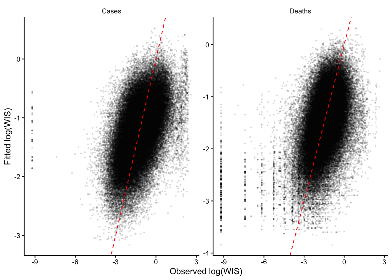
Despite the improved residual behaviour, the substantive conclusions are unchanged. The model-structure and geographic-scope effects remain centred on zero under both specifications (the headline finding of no systematic structural difference is identical), and the direction of every covariate effect is preserved (correlation of adjusted partial effects ≈ 0.96 across the focal covariates). The magnitudes of some target-difficulty effects are attenuated on the log-response scale — for example the stable-trend advantage is smaller — reflecting the different treatment of the skewed upper tail, but no effect changes sign. We therefore retain the log-link specification in the main text for continuity with the scoring scale and report this transformation as a robustness check.