Forecasting Models Guide

library(forecastbaselines)
#> Julia version 1.11.9 at location /opt/hostedtoolcache/julia/1.11.9/x64/bin will be used.
#> Loading setup script for JuliaCall...
#> Finish loading setup script for JuliaCall.
#> forecastbaselines: Julia backend loaded successfully
library(scoringutils)
library(ggplot2)
setup_ForecastBaselines()
#> Initializing Julia...
#> Julia initialized successfully
#> Checking ForecastBaselines.jl installation...
#> ForecastBaselines.jl is already installed
#> Loading R conversion helpers...
#> forecastbaselines setup complete!

Overview

forecastbaselines provides 10 baseline forecasting models across three categories:

Simple Baselines - Naive methods for benchmarking
Seasonal/Trend Models - For patterned data
Advanced Time Series Models - Statistical models

This vignette provides:

Detailed description of each model
When to use each model
Parameter guidance
Practical examples
Performance characteristics

Model Selection Guide

Quick Decision Tree

Do you have seasonal patterns?
├─ Yes, strong seasonality
│  ├─ Regular pattern → STLModel(s = period)
│  ├─ Irregular pattern → LSDModel(window_width, s = period)
│  └─ Need decomposition → STLModel(s = period)
├─ No, mostly trend
│  ├─ Polynomial trend → OLSModel(degree)
│  ├─ Step changes → IDSModel(window_size)
│  └─ Complex trend → ARMAModel(p, q)
└─ No clear pattern
   ├─ Need simple baseline → ConstantModel()
   ├─ Sample from history → MarginalModel()
   └─ Smooth estimates → KDEModel()

Special cases:
- Count data (integers) → INARCHModel(p)
- Multiple components → ETSModel(error_type, trend_type, season_type)
- Quick benchmark → ConstantModel()

Model Comparison Table

Model	Complexity	Data Needs	Seasonality	Trend	Prob. Forecasts
Constant	Very Low	Minimal (1+)	No	No	Via residuals
Marginal	Very Low	30+	No	No	Direct
KDE	Low	50+	No	No	Direct
LSD	Low	2+ cycles	Yes	No	Via residuals
OLS	Low	20+	No	Yes	Via residuals
IDS	Low	20+	No	Yes	Via residuals
STL	Medium	2+ cycles	Yes	Yes	Via residuals
ARMA	Medium	50+	No	No	Parametric
INARCH	Medium	50+	Yes	No	Parametric
ETS	High	50+	Yes	Yes	Parametric

1. Simple Baseline Models

These models provide quick, interpretable forecasts and serve as benchmarks for more complex methods.

1.1 Constant Model (Naive Forecast)

Description: The simplest possible forecast - uses the last observed value for all future predictions.

Mathematical Form: $\hat{y}_{t+h} = y_t \quad \forall h > 0$

When to Use:

✅ Quick baseline for model comparison
✅ Random walk data (financial prices, etc.)
✅ When you need fast, simple forecasts
❌ Data with trends or seasonality

Parameters: None - completely parameter-free.

Example:

# Generate random walk data
set.seed(123)
data <- cumsum(rnorm(100))

# Fit constant model
model <- ConstantModel()
fitted <- fit_baseline(data, model)

# Forecast
fc <- forecast(fitted, interval_method = NoInterval(), horizon = 1:10)

# Visualize
n_data <- length(data)
plot_df <- rbind(
  data.frame(time = 1:n_data, value = data, type = "Observed"),
  data.frame(time = 101:110, value = fc$mean, type = "Forecast")
)

ggplot(plot_df, aes(x = time, y = value)) +
  geom_line(aes(color = type), linewidth = 1) +
  geom_hline(yintercept = data[100], linetype = "dashed", color = "red", alpha = 0.5) +
  scale_color_manual(values = c("Observed" = "black", "Forecast" = "red")) +
  labs(title = "Constant Model: Random Walk Forecast", x = "Time", y = "Value", color = NULL) +
  theme_minimal() +
  theme(legend.position = "top")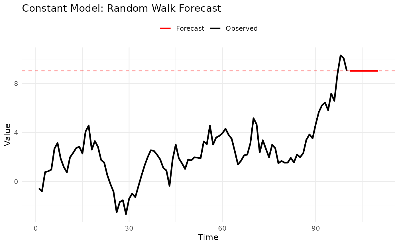

Strengths:

Extremely fast
No parameters to tune
Optimal for random walks
Easy to explain

Limitations:

Ignores all patterns
Flat forecast function
Poor for trending/seasonal data

1.2 Marginal Model

Description: Forecasts by randomly sampling from the empirical distribution of the observed data.

Mathematical Form: $\hat{y}_{t+h} \sim \text{Empirical}(y_1, \ldots, y_t)$

When to Use:

✅ Stationary data without autocorrelation
✅ Need probabilistic forecasts
✅ Distribution shape matters more than sequence
❌ Trending or seasonal patterns
❌ Strong autocorrelation

Parameters: None

Example:

# Generate stationary data
set.seed(123)
data <- rnorm(100, mean = 50, sd = 10)

# Fit marginal model
model <- MarginalModel()
fitted <- fit_baseline(data, model)

# Forecast with prediction intervals
fc <- forecast(
  fitted,
  interval_method = EmpiricalInterval(n_trajectories = 1000),
  horizon = 1:10,
  levels = c(0.5, 0.95),
  model_name = "Marginal"
)

# The forecast mean approximates the historical mean
cat("Historical mean:", mean(data), "\n")
#> Historical mean: 50.90406
cat("Forecast mean:", mean(fc$mean), "\n")
#> Forecast mean: 50.90406

# Quantile forecasts are now available for scoring
set.seed(124)
truth <- 50 + rnorm(10, 0, 10)  # Simulated future values
fc_truth <- add_truth(fc, truth)

# Convert to quantile format and show structure
fc_quantile <- scoringutils::as_forecast_quantile(fc_truth)
print(head(fc_quantile, 15))  # Show first few quantiles
#>     observed predicted quantile_level horizon    model
#>        <num>     <num>          <num>   <int>   <char>
#>  1: 36.14929  33.76226          0.025       1 Marginal
#>  2: 36.14929  45.17317          0.250       1 Marginal
#>  3: 36.14929  50.23163          0.500       1 Marginal
#>  4: 36.14929  57.15998          0.750       1 Marginal
#>  5: 36.14929  70.45712          0.975       1 Marginal
#>  6: 50.38323  33.76226          0.025       2 Marginal
#>  7: 50.38323  44.43653          0.250       2 Marginal
#>  8: 50.38323  50.23163          0.500       2 Marginal
#>  9: 50.38323  57.22381          0.750       2 Marginal
#> 10: 50.38323  70.44441          0.975       2 Marginal
#> 11: 42.36970  34.37043          0.025       3 Marginal
#> 12: 42.36970  45.12309          0.250       3 Marginal
#> 13: 42.36970  51.04169          0.500       3 Marginal
#> 14: 42.36970  58.49046          0.750       3 Marginal
#> 15: 42.36970  70.44441          0.975       3 Marginal

Strengths:

Captures full distribution
Natural uncertainty quantification
No distributional assumptions

Limitations:

Ignores temporal dependence
Requires sufficient data (30+)
Constant forecast on average

Use Case: Benchmark for comparing autocorrelation benefits. If ARMA doesn’t beat Marginal, your data may not have useful autocorrelation.

1.3 KDE Model (Kernel Density Estimation)

Description: Similar to Marginal but uses kernel density estimation for smoother probability distributions.

Mathematical Form: $\hat{f}(y) = \frac{1}{n h} \sum_{i=1}^n K\left(\frac{y - y_i}{h}\right)$

where $K$ is a kernel function and $h$ is bandwidth.

When to Use:

✅ Need smooth probability estimates
✅ Continuous data
✅ Multi-modal distributions
❌ Small sample sizes (< 50)
❌ Discrete/count data

Parameters: None (bandwidth selected automatically)

Example:

# Generate bimodal data
set.seed(123)
data <- c(
  rnorm(50, mean = 20, sd = 3),
  rnorm(50, mean = 40, sd = 3)
)

# Compare Marginal vs KDE
marginal <- fit_baseline(data, MarginalModel())
kde <- fit_baseline(data, KDEModel())

fc_marginal <- forecast(marginal, interval_method = NoInterval(), horizon = 1:100)
fc_kde <- forecast(kde, interval_method = NoInterval(), horizon = 1:100)

# KDE produces smoother samples
# Prepare data for ggplot
marginal_density <- density(fc_marginal$mean)
kde_density <- density(fc_kde$mean)

density_df <- rbind(
  data.frame(x = marginal_density$x, y = marginal_density$y, type = "Marginal"),
  data.frame(x = kde_density$x, y = kde_density$y, type = "KDE")
)

ggplot(density_df, aes(x = x, y = y, color = type)) +
  geom_line(linewidth = 1.5) +
  scale_color_manual(values = c("Marginal" = "red", "KDE" = "blue")) +
  labs(title = "Marginal vs KDE", x = "Forecast Value", y = "Density", color = NULL) +
  theme_minimal() +
  theme(legend.position = "topright")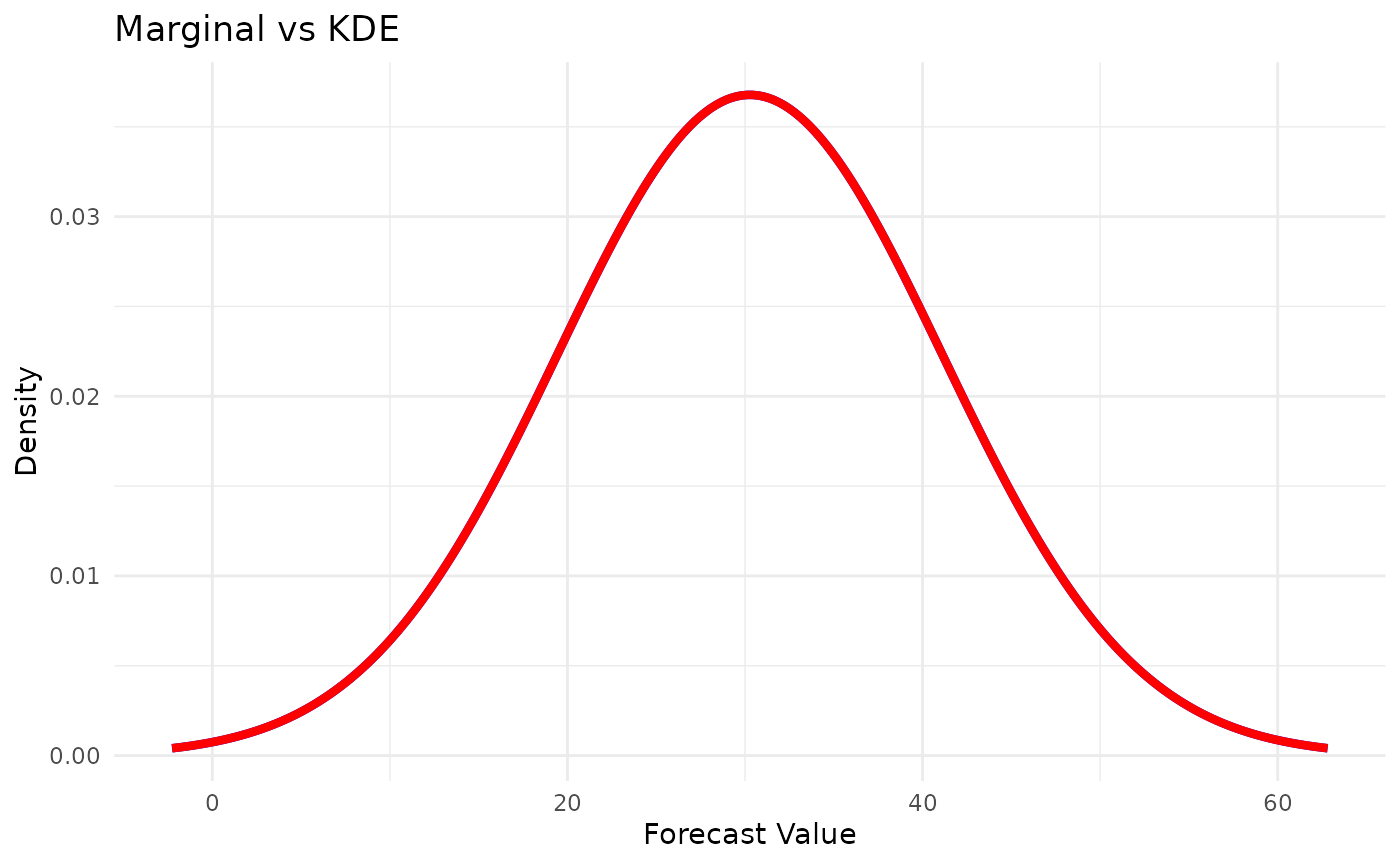

Strengths:

Smooth probability estimates
Handles multi-modal data
Good for continuous distributions

Limitations:

Needs more data than Marginal (50+)
Computationally more expensive
Still ignores autocorrelation

2. Seasonal and Trend Models

For data with identifiable patterns in time.

2.1 LSD Model (Last Similar Dates)

Description: Seasonal model that forecasts by averaging values from similar historical periods.

How It Works:

For horizon $h$ , look back to periods $t - s + h$ , $t - 2s + h$ , etc.
Average the window most recent similar periods
Handles irregular seasonality well

When to Use:

✅ Strong seasonal patterns
✅ Seasonality more important than trend
✅ Irregular seasonal effects
❌ Purely trending data
❌ Less than 2 full seasonal cycles

Parameters:

window: Number of similar periods to average (default: 1)
s: Seasonal period (e.g., 12 for monthly, 7 for daily)

Example:

# Monthly data with seasonality
set.seed(123)
months <- 1:240
seasonal_pattern <- 20 + 10 * sin(2 * pi * months / 12)
data <- seasonal_pattern + rnorm(240, sd = 2)

# Fit LSD model
model <- LSDModel(window_width = 3, s = 12) # Average last 3 years
fitted <- fit_baseline(data, model)

# Forecast next year
fc <- forecast(fitted, interval_method = NoInterval(), horizon = 1:12)

# Plot
n_data <- length(data)
plot_df <- rbind(
  data.frame(time = 1:n_data, value = data, type = "Observed"),
  data.frame(time = 241:252, value = fc$mean, type = "Forecast")
)

ggplot(plot_df, aes(x = time, y = value, color = type)) +
  geom_line(linewidth = 1) +
  scale_color_manual(values = c("Observed" = "black", "Forecast" = "red")) +
  labs(title = "LSD Model: Seasonal Forecast", x = "Time", y = "Value", color = NULL) +
  theme_minimal() +
  theme(legend.position = "top")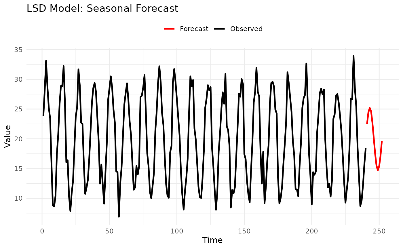

Parameter Guidance:

s (seasonal period):
- 7 for daily data with weekly patterns
- 12 for monthly data with yearly patterns
- 24 for hourly data with daily patterns
- 52 for weekly data with yearly patterns
window (averaging window):
- 1: Use only last similar period (more responsive)
- 3-5: Smooth average (more stable)
- Large: Very smooth but less adaptive

Strengths:

Simple and interpretable
Handles irregular seasonality
Fast computation
Works with little data

Limitations:

No trend modeling
Needs at least 2 seasonal cycles
Fixed seasonal period

2.2 OLS Model (Polynomial Trend)

Description: Fits polynomial trends using ordinary least squares, then forecasts by extrapolating the trend.

Mathematical Form: $y_t = \beta_0 + \beta_1 t + \beta_2 t^2 + \ldots + \beta_p t^p + \epsilon_t$

When to Use:

✅ Clear polynomial trends
✅ Smooth, continuous trends
✅ Short-term extrapolation
❌ Seasonal patterns
❌ Long-term forecasts (unstable extrapolation)

Parameters:

degree: Polynomial degree (1 = linear, 2 = quadratic, etc.)
differencing: Order of differencing (default: 0)

Example:

# Generate quadratic trend
set.seed(123)
time <- 1:50
data <- 10 + 2 * time + 0.05 * time^2 + rnorm(50, sd = 3)

# Compare linear vs quadratic
linear <- fit_baseline(data, OLSModel(degree = 1))
quadratic <- fit_baseline(data, OLSModel(degree = 2))

fc_linear <- forecast(linear, interval_method = NoInterval(), horizon = 1:10)
fc_quadratic <- forecast(quadratic, interval_method = NoInterval(), horizon = 1:10)

# Plot
n_data <- length(data)
plot_df <- rbind(
  data.frame(time = 1:n_data, value = data, type = "Data"),
  data.frame(time = 51:60, value = fc_linear$mean, type = "Linear"),
  data.frame(time = 51:60, value = fc_quadratic$mean, type = "Quadratic")
)

ggplot(plot_df, aes(x = time, y = value, color = type)) +
  geom_line(aes(linewidth = type)) +
  scale_linewidth_manual(values = c("Data" = 0.5, "Linear" = 1, "Quadratic" = 1)) +
  scale_color_manual(values = c("Data" = "black", "Linear" = "blue", "Quadratic" = "red")) +
  labs(title = "OLS: Linear vs Quadratic Trend", x = "Time", y = "Value", color = NULL, linewidth = NULL) +
  theme_minimal() +
  theme(legend.position = "top")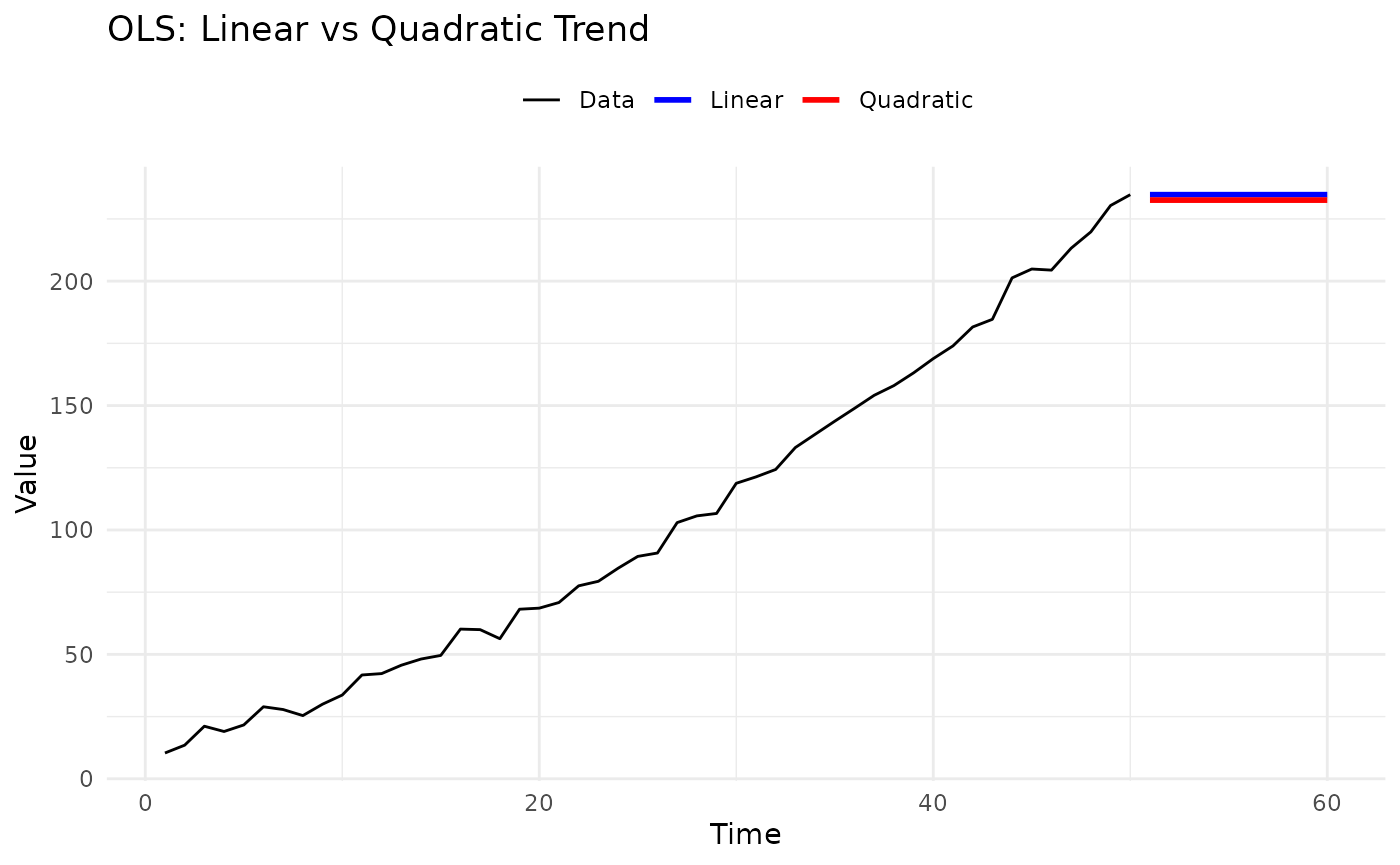

Parameter Guidance:

degree:
- 1: Linear trend (most common)
- 2: Quadratic (turning point)
- 3: Cubic (S-shaped curves)
- 4+: Rarely recommended (overfitting risk)
differencing:
- 0: Model in levels
- 1: Model in first differences
- Requires degree >= differencing + 1

Strengths:

Simple interpretation
Fast computation
Well-understood statistics

Limitations:

Polynomial extrapolation can be unstable
No seasonality handling
Overfitting risk with high degrees

Tips:

Use degree = 1 (linear) unless there’s clear curvature
Validate extrapolations carefully
Consider ARMA for long-term forecasts

2.3 IDS Model (Increase-Decrease-Stable)

Description: Detects trend direction (increasing, decreasing, stable) over recent windows and extrapolates.

How It Works:

Divide recent history into p windows
Classify each window’s trend
Forecast based on detected pattern

When to Use:

✅ Step changes in trend
✅ Regime-switching behavior
✅ Need trend detection
❌ Smooth continuous trends (use OLS)
❌ Seasonal patterns

Parameters:

window_size: Number of windows to analyze (default: 3)
threshold: Threshold for detecting changes (default: 0.0)

Example:

# Generate data with trend change
set.seed(123)
data <- c(
  seq(10, 30, length.out = 30), # Increasing
  rep(30, 20) + rnorm(20, sd = 1), # Stable
  seq(30, 50, length.out = 30) # Increasing again
)

# Fit IDS model
model <- IDSModel(window_size = 3) # Analyze last 3 windows
fitted <- fit_baseline(data, model)

# Forecast
fc <- forecast(fitted, interval_method = NoInterval(), horizon = 1:15)

# Plot
n_data <- length(data)
plot_df <- rbind(
  data.frame(time = 1:n_data, value = data, type = "Observed"),
  data.frame(time = 81:95, value = fc$mean, type = "Forecast")
)

ggplot(plot_df, aes(x = time, y = value, color = type)) +
  geom_line(linewidth = 1) +
  geom_vline(xintercept = c(30, 50), linetype = "dashed", alpha = 0.5) +
  scale_color_manual(values = c("Observed" = "black", "Forecast" = "red")) +
  labs(title = "IDS Model: Trend Detection", x = "Time", y = "Value", color = NULL) +
  theme_minimal() +
  theme(legend.position = "top")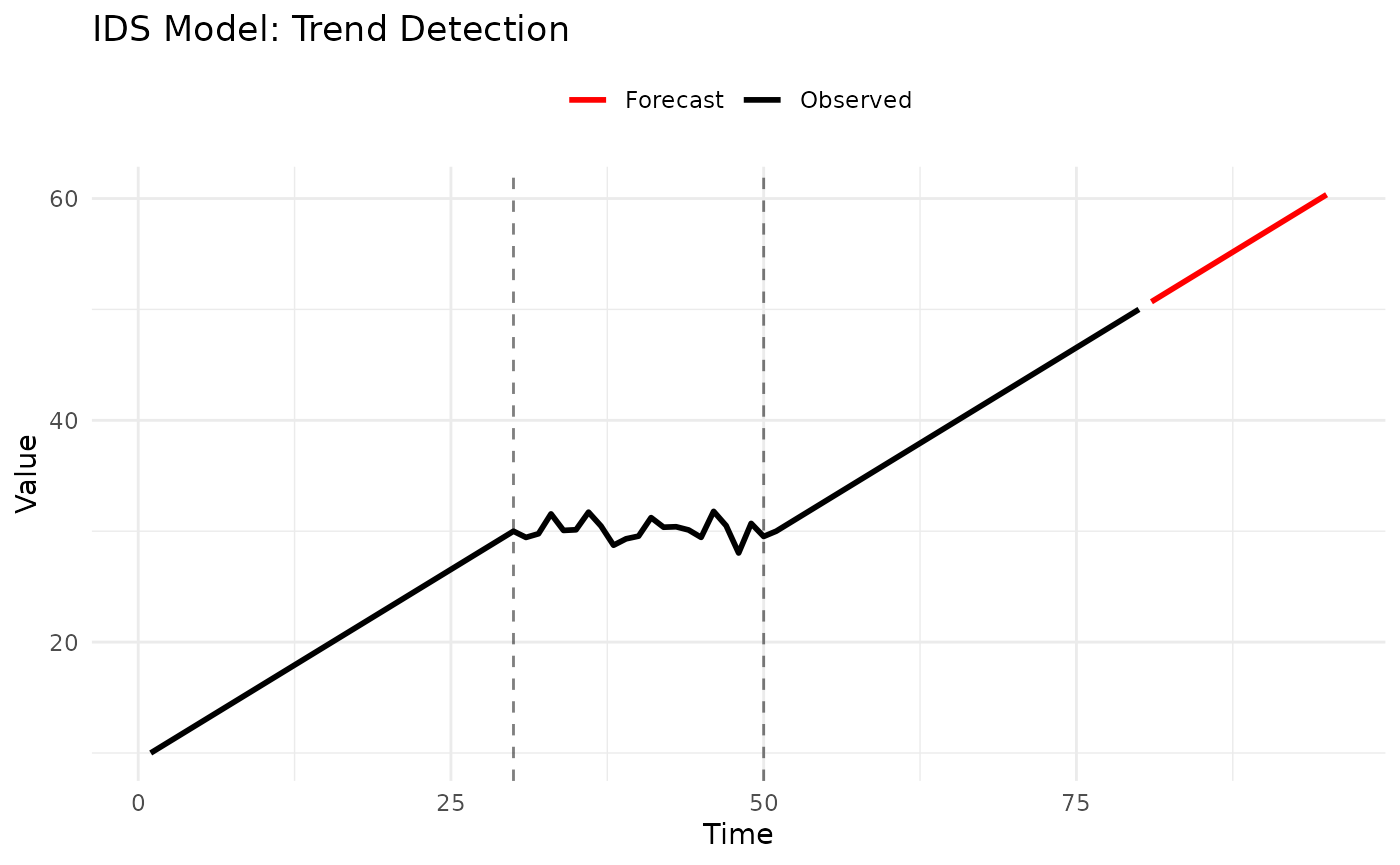

Parameter Guidance:

p (number of windows):
- 2-3: More reactive to recent changes
- 4-6: More stable, less reactive
- Too large: Misses recent trends

Strengths:

Detects trend changes
Adapts to regimes
Interpretable classifications

Limitations:

Discrete trend categories
Needs sufficient data
No seasonality

2.4 STL Model (Seasonal-Trend Decomposition)

Description: Decomposes series into seasonal, trend, and remainder components using LOESS, then forecasts each separately.

Mathematical Form: $y_t = T_t + S_t + R_t$

where $T_t$ is trend, $S_t$ is seasonal, $R_t$ is remainder.

When to Use:

✅ Both trend AND seasonality
✅ Need decomposition for interpretation
✅ Regular seasonal patterns
❌ Irregular seasonality
❌ Less than 2 seasonal cycles

Parameters:

s: Seasonal period

Example:

# Generate trend + seasonality
set.seed(123)
time <- 1:240 # 20 years of monthly data
trend <- 0.5 * time
seasonal <- 10 * sin(2 * pi * time / 12)
data <- 50 + trend + seasonal + rnorm(240, sd = 2)

# Fit STL model
model <- STLModel(s = 12)
fitted <- fit_baseline(data, model)

# Forecast next year
fc <- forecast(fitted, interval_method = NoInterval(), horizon = 1:12)

# Plot
n_data <- length(data)
plot_df <- rbind(
  data.frame(time = 1:n_data, value = data, type = "Observed"),
  data.frame(time = 241:252, value = fc$mean, type = "Forecast")
)

ggplot(plot_df, aes(x = time, y = value, color = type)) +
  geom_line(linewidth = 1) +
  scale_color_manual(values = c("Observed" = "black", "Forecast" = "red")) +
  labs(title = "STL Model: Trend + Seasonality", x = "Time", y = "Value", color = NULL) +
  theme_minimal() +
  theme(legend.position = "top")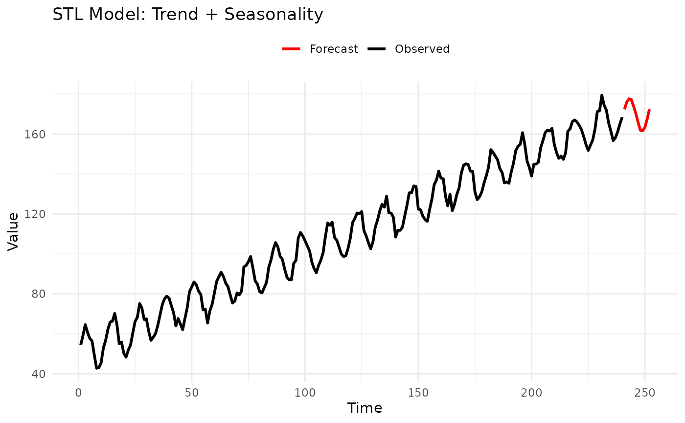

Parameter Guidance:

s (seasonal period): Same as LSD model guidance

Strengths:

Handles trend + seasonality together
Robust to outliers
Provides interpretable decomposition
Can extract components for analysis

Limitations:

Fixed seasonal period
Needs at least 2 cycles
More complex than LSD

Use Case: Preferred over LSD when trend is important, or when you need to analyze seasonal and trend components separately.

3. Advanced Time Series Models

Statistical models with parametric probability distributions.

3.1 ARMA Model (Autoregressive Moving Average)

Description: Classic time series model combining autoregressive (AR) and moving average (MA) components.

Mathematical Form: $y_t = c + \phi_1 y_{t-1} + \ldots + \phi_p y_{t-p} + \theta_1 \epsilon_{t-1} + \ldots + \theta_q \epsilon_{t-q} + \epsilon_t$

where $\epsilon_t \sim N(0, \sigma^2)$ .

When to Use:

✅ Stationary time series
✅ Need parametric uncertainty
✅ Autocorrelation structure
❌ Strong trends (use differencing or detrend first)
❌ Seasonal patterns (use SARIMA or seasonal models)

Parameters:

p: Autoregressive order
q: Moving average order

Example:

# Generate AR(1) process
set.seed(123)
n <- 200
data <- numeric(n)
data[1] <- rnorm(1)
for (i in 2:n) {
  data[i] <- 0.7 * data[i - 1] + rnorm(1)
}

# Fit ARMA(2,1)
model <- ARMAModel(p = 2, q = 1)
fitted <- fit_baseline(data, model)

# Forecast with prediction intervals
fc <- forecast(
  fitted,
  interval_method = EmpiricalInterval(n_trajectories = 1000),
  horizon = 1:20,
  levels = c(0.5, 0.95),
  model_name = "ARMA(2,1)"
)

# Add simulated truth and visualize with intervals
set.seed(456)
truth <- numeric(20)
truth[1] <- 0.7 * data[200] + rnorm(1)
for (i in 2:20) {
  truth[i] <- 0.7 * truth[i - 1] + rnorm(1)
}

fc_truth <- add_truth(fc, truth)
fc_quantile <- scoringutils::as_forecast_quantile(fc_truth)

# Show quantile forecast structure
print(head(fc_quantile, 15))
#>        observed  predicted quantile_level horizon     model
#>           <num>      <num>          <num>   <int>    <char>
#>  1: -2.64651490 -3.0532104          0.025       1 ARMA(2,1)
#>  2: -2.64651490 -1.8735702          0.250       1 ARMA(2,1)
#>  3: -2.64651490 -1.2528488          0.500       1 ARMA(2,1)
#>  4: -2.64651490 -0.5709904          0.750       1 ARMA(2,1)
#>  5: -2.64651490  1.2804917          0.975       1 ARMA(2,1)
#>  6: -1.23078488 -2.5489403          0.025       2 ARMA(2,1)
#>  7: -1.23078488 -1.3998319          0.250       2 ARMA(2,1)
#>  8: -1.23078488 -0.8751294          0.500       2 ARMA(2,1)
#>  9: -1.23078488 -0.1682574          0.750       2 ARMA(2,1)
#> 10: -1.23078488  1.7020715          0.975       2 ARMA(2,1)
#> 11: -0.06067475 -2.3424184          0.025       3 ARMA(2,1)
#> 12: -0.06067475 -1.0874471          0.250       3 ARMA(2,1)
#> 13: -0.06067475 -0.4711444          0.500       3 ARMA(2,1)
#> 14: -0.06067475  0.2061740          0.750       3 ARMA(2,1)
#> 15: -0.06067475  1.6094645          0.975       3 ARMA(2,1)

Parameter Guidance:

How to choose p and q:

Plot ACF/PACF (in R):

acf(data) # Autocorrelation
pacf(data) # Partial autocorrelation

ACF/PACF patterns:
- ACF cuts off at lag q → MA(q)
- PACF cuts off at lag p → AR(p)
- Both decay slowly → ARMA(p,q)
Common starting points:
- ARMA(1,0) = AR(1): Simple persistence
- ARMA(0,1) = MA(1): Single shock memory
- ARMA(1,1): Most parsimonious mixed model
- ARMA(2,2): More flexibility
General guidance:
- Start small (p=1, q=1)
- Rarely need p or q > 3
- More parameters ≠ better forecasts

Strengths:

Well-established theory
Parametric uncertainty
Efficient for stationary data
Many diagnostic tools

Limitations:

Requires stationarity
Parameter selection can be tricky
Needs sufficient data (50+)

Tips:

Detrend before fitting if trending
Use AIC/BIC for model selection
Check residuals for white noise

3.2 INARCH Model (Integer ARCH)

Description: Designed for count data (non-negative integers), models conditional mean and variance with ARCH-type dynamics.

Mathematical Form: $E[y_t | \mathcal{F}_{t-1}] = \beta + \alpha_1 y_{t-1} + \ldots + \alpha_p y_{t-p}$ $y_t | \mathcal{F}_{t-1} \sim \text{Poisson}(\lambda_t)$

When to Use:

✅ Count data (0, 1, 2, 3, …)
✅ Non-negative integers
✅ Overdispersion
✅ Time-varying variance
❌ Continuous data
❌ Negative values

Parameters:

p: Order of lags
s: Seasonal period (optional)

Example:

# Generate count data
set.seed(123)
# Simulate Poisson AR process
lambda <- 10
data <- numeric(100)
data[1] <- rpois(1, lambda)
for (i in 2:100) {
  mu <- 5 + 0.5 * data[i - 1]
  data[i] <- rpois(1, mu)
}

# Fit INARCH(1)
model <- INARCHModel(p = 1)
fitted <- fit_baseline(data, model)

# Forecast
fc <- forecast(fitted, interval_method = NoInterval(), horizon = 1:10)

# Forecasts are counts
print(fc$mean)
#>  [1] 8.771931 9.145271 9.325835 9.413164 9.455401 9.475828 9.485708 9.490486
#>  [9] 9.492797 9.493915

Parameter Guidance:

p (lag order):
- 1: Most common, captures direct persistence
- 2-3: If ACF shows higher-order dependence
- Rarely need p > 3
s (seasonality):
- Omit if no seasonality
- Set to period if seasonal counts

Strengths:

Designed for count data
Respects non-negativity
Handles overdispersion
Seasonal version available

Limitations:

Only for integer counts
Requires more data than ARMA
Limited to Poisson/NegBin distributions

Use Cases:

Disease counts
Customer arrivals
Event occurrences
Web traffic hits

3.3 ETS Model (Error-Trend-Season)

Description: Exponential smoothing state space models covering 30 different combinations of error, trend, and seasonal components.

Components:

Error: Additive (A) or Multiplicative (M)
Trend: None (N), Additive (A), Multiplicative (M), Damped (Ad, Md)
Season: None (N), Additive (A), Multiplicative (M)

When to Use:

✅ Complex seasonal patterns
✅ Need automatic model selection
✅ Business forecasting
✅ Various data characteristics
❌ Very short series (< 2 cycles)
❌ Need interpretable parameters

Parameters:

error: “A” (additive) or “M” (multiplicative) or NULL (auto)
trend: “N”, “A”, “M”, “Ad”, “Md”, or NULL (auto)
season: “N”, “A”, “M”, or NULL (auto)
s: Seasonal period (if seasonal)

Example:

# Generate multiplicative seasonal data
set.seed(123)
time <- 1:72
trend <- 100 + 2 * time
seasonal_mult <- 1 + 0.3 * sin(2 * pi * time / 12)
data <- trend * seasonal_mult * exp(rnorm(72, sd = 0.05))

# Automatic selection
model_auto <- ETSModel()
fitted_auto <- fit_baseline(data, model_auto)

# Specific: Multiplicative error, additive trend, multiplicative season
model_specific <- ETSModel(error_type = "M", trend_type = "A", season_type = "M", s = 12)
fitted_specific <- fit_baseline(data, model_specific)

# Forecast
fc <- forecast(fitted_specific,
  interval_method = NoInterval(),
  horizon = 1:12
)

# Plot
n_data <- length(data)
plot_df <- rbind(
  data.frame(time = 1:n_data, value = data, type = "Observed"),
  data.frame(time = 73:84, value = fc$mean, type = "Forecast")
)

ggplot(plot_df, aes(x = time, y = value, color = type)) +
  geom_line(linewidth = 1) +
  scale_color_manual(values = c("Observed" = "black", "Forecast" = "red")) +
  labs(title = "ETS Model: Complex Seasonality", x = "Time", y = "Value", color = NULL) +
  theme_minimal() +
  theme(legend.position = "top")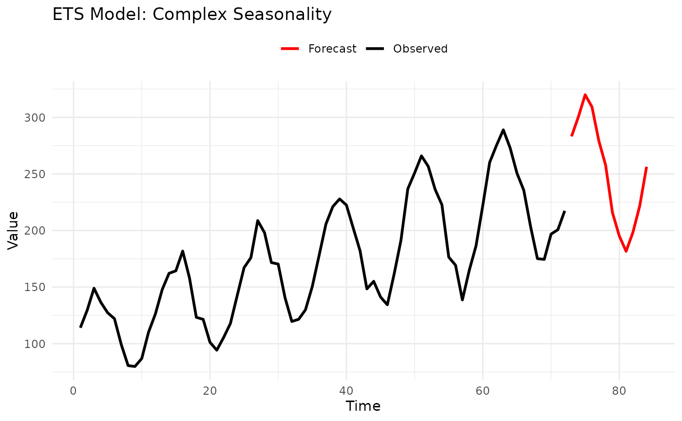

Model Selection Guide:

Error type:

Additive (A): Errors independent of level
Multiplicative (M): Errors proportional to level

Trend type:

None (N): No trend
Additive (A): Linear trend
Multiplicative (M): Exponential trend
Additive Damped (Ad): Trend decays to flat
Multiplicative Damped (Md): Trend decays exponentially

Season type:

None (N): No seasonality
Additive (A): Constant seasonal fluctuation
Multiplicative (M): Seasonal % of level

Common Models:

ETS(A,N,N): Simple exponential smoothing
ETS(A,A,N): Holt’s linear trend
ETS(A,A,A): Additive Holt-Winters
ETS(A,A,M): Multiplicative seasonality
ETS(M,M,M): Fully multiplicative

Strengths:

Extremely flexible (30 models)
Automatic selection available
Well-tested in practice
Handles many data types

Limitations:

Many parameters to choose
Computationally intensive
Less interpretable than ARMA
Can overfit

Tips:

Start with automatic selection (NULL parameters)
Use additive for stable variance
Use multiplicative for percentage seasonality
Damped trends for long horizons

Model Selection Examples

Example 1: Monthly Sales Data

# Simulated retail sales: trend + seasonality + promotions
set.seed(123)
months <- 1:240
trend <- 1000 + 20 * months
seasonal <- 200 * sin(2 * pi * months / 12) # Holiday peaks
noise <- rnorm(240, sd = 50)
data <- trend + seasonal + noise

# Try multiple models
models <- list(
  Naive = ConstantModel(),
  LSD = LSDModel(window_width = 3, s = 12),
  STL = STLModel(s = 12),
  ETS = ETSModel(error_type = "A", trend_type = "A", season_type = "A", s = 12)
)

# Fit all models
results <- lapply(names(models), function(name) {
  fitted <- fit_baseline(data, models[[name]])
  fc <- forecast(fitted, interval_method = NoInterval(), horizon = 1:12)

  data.frame(
    Model = name,
    Forecast_Mean = mean(fc$mean)
  )
})

comparison <- do.call(rbind, results)
print(comparison)
#>   Model Forecast_Mean
#> 1 Naive      5760.923
#> 2   LSD      3417.800
#> 3   STL      5858.771
#> 4   ETS      5924.238

# Recommendation: STL or ETS for trend + seasonality

Example 2: Website Traffic (Count Data)

# Daily page views (count data)
set.seed(456)
days <- 100
data <- rpois(days, lambda = 100 + 0.5 * 1:days)

# Count-specific models
models <- list(
  Marginal = MarginalModel(), # Ignore trend
  INARCH = INARCHModel(p = 1) # Model count dynamics
)

# Compare
# INARCH should perform better due to trend

# Recommendation: INARCH for count data with patterns

Example 3: Financial Returns

# Daily returns (stationary, no trend/season)
set.seed(789)
data <- rnorm(200, mean = 0.001, sd = 0.02)

# Stationary models
models <- list(
  Marginal = MarginalModel(),
  ARMA = ARMAModel(p = 1, q = 1)
)

# For returns, ARMA captures autocorrelation
# Marginal is baseline

# Recommendation: ARMA if autocorrelation present, else Marginal

Performance Considerations

Computational Speed (Relative)

Fastest → Slowest:

ConstantModel (instant)
MarginalModel, KDEModel (very fast)
LSDModel, OLSModel, IDSModel (fast)
STLModel, ARMAModel (moderate)
INARCHModel, ETSModel (slower)

Data Requirements (Minimum)

Model	Absolute Min	Recommended
Constant	1	20+
Marginal	20	50+
KDE	30	100+
LSD	2*s	3*s+
OLS	degree+1	30+
IDS	10	30+
STL	2*s	3*s+
ARMA	p+q	50+
INARCH	20	50+
ETS	2*s (if seasonal)	50+

Summary and Recommendations

Quick Start

Don’t know where to begin?

Start with ConstantModel() - it’s fast and shows what “no model” looks like
If you have seasonality, try STLModel(s = period)
If stationary without seasonality, try ARMAModel(p = 1, q = 1)
Compare models with score() functions

Best Practices

Always use a simple baseline - ConstantModel or Marginal
Match model to data characteristics:
- Counts → INARCH
- Seasonal → STL or LSD
- Stationary → ARMA
- Complex → ETS
Validate on holdout data - use truth parameter
Check residuals - should look like white noise
Start simple, add complexity only if needed

Appendix: Parameter Quick Reference

# Simple Baselines
ConstantModel()
MarginalModel()
KDEModel()

# Seasonal/Trend
LSDModel(window_width = 3, s = 12)
OLSModel(degree = 1, differencing = 0)
IDSModel(window_size = 3)
STLModel(s = 12)

# Advanced
ARMAModel(p = 1, q = 1)
INARCHModel(p = 1, s = NULL)
ETSModel(error_type = "A", trend_type = "N", season_type = "N", s = NULL)

Overview

Model Selection Guide

Quick Decision Tree

Model Comparison Table

1. Simple Baseline Models

1.1 Constant Model (Naive Forecast)

1.2 Marginal Model

1.3 KDE Model (Kernel Density Estimation)

2. Seasonal and Trend Models

2.1 LSD Model (Last Similar Dates)

2.2 OLS Model (Polynomial Trend)

2.3 IDS Model (Increase-Decrease-Stable)

2.4 STL Model (Seasonal-Trend Decomposition)

3. Advanced Time Series Models

3.1 ARMA Model (Autoregressive Moving Average)

3.2 INARCH Model (Integer ARCH)

3.3 ETS Model (Error-Trend-Season)

Model Selection Examples

Example 1: Monthly Sales Data

Example 2: Website Traffic (Count Data)

Example 3: Financial Returns

Performance Considerations

Computational Speed (Relative)

Data Requirements (Minimum)

Summary and Recommendations

Quick Start

Best Practices

Further Reading

Appendix: Parameter Quick Reference