Getting Started with forecastbaselines
Source:vignettes/forecastbaselines.Rmd
forecastbaselines.RmdIntroduction
forecastbaselines provides an R interface to the ForecastBaselines.jl Julia package, giving you access to 10 baseline forecasting models with uncertainty quantification and evaluation tools.
This vignette will walk you through:
- Installation and setup
- Your first forecast
- Probabilistic forecasting with prediction intervals
- Model evaluation and scoring
- Next steps
Installation
Prerequisites
You’ll need both Julia and R installed:
Julia (>= 1.9)
- Download from julialang.org
- Verify installation:
julia --version
R (>= 3.5.0)
- Already installed if you’re reading this!
Install forecastbaselines
# Install from GitHub
# install.packages("remotes")
remotes::install_github("epiforecasts/forecastbaselines")
Setup Julia Backend
The first time you use the package, you need to set up the Julia backend:
library(forecastbaselines)
#> Julia version 1.11.9 at location /opt/hostedtoolcache/julia/1.11.9/x64/bin will be used.
#> Loading setup script for JuliaCall...
#> Finish loading setup script for JuliaCall.
#> forecastbaselines: Julia backend loaded successfully
library(scoringutils)
library(ggplot2)

# One-time setup: installs Julia packages
setup_ForecastBaselines()
#> Initializing Julia...
#> Julia initialized successfully
#> Checking ForecastBaselines.jl installation...
#> ForecastBaselines.jl is already installed
#> Loading R conversion helpers...
#> forecastbaselines setup complete!
This will:
- Initialize Julia from R
- Install the ForecastBaselines.jl package
- Install all dependencies
- Load helper functions
Note: This only needs to be done once. Subsequent R sessions will automatically connect to Julia.
Your First Forecast
Let’s create a simple forecast using the Constant (naive) model, which uses the last observed value as the forecast.
Generate Some Data
# Simulate a time series with trend and seasonality
set.seed(123)
n_total <- 62  # Total observations
n_train <- 50  # Training set size
time <- 1:n_total
trend <- 0.5 * time
seasonal <- 5 * sin(2 * pi * time / 12)
noise <- rnorm(n_total, sd = 2)
full_data <- trend + seasonal + noise

# Split into training and test sets
data <- full_data[1:n_train]
truth <- full_data[(n_train + 1):n_total]

# Plot the full series
plot_df <- data.frame(
  time = 1:n_total,
  value = full_data,
  set = c(rep("Training", n_train), rep("Test", n_total - n_train))
)

ggplot(plot_df, aes(x = time, y = value, color = set)) +
  geom_line() +
  labs(title = "Simulated Time Series", x = "Time", y = "Value") +
  theme_minimal()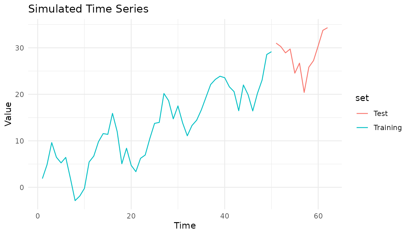
Fit a Model
# Create a Constant (naive) model
model <- ConstantModel()

# Fit the model to the data
fitted <- fit_baseline(data, model)
Generate Forecasts
# Forecast 12 steps ahead
horizon <- 1:12
fc <- forecast(fitted,
  interval_method = NoInterval(),
  horizon = horizon
)

# View the forecast
print(fc)
#> ForecastBaselines Forecast Object
#> ==================================
#>
#> Horizon: 1 to 12
#>
#> Components:
#>   - Mean forecasts
#>   - Median forecasts

# Access forecast values
fc$mean
#>  [1] 29.16339 29.16339 29.16339 29.16339 29.16339 29.16339 29.16339 29.16339
#>  [9] 29.16339 29.16339 29.16339 29.16339
Visualize Results
# Plot data and forecast
plot_df <- rbind(
  data.frame(time = 1:n_train, value = data, type = "Observed"),
  data.frame(time = (n_train + 1):(n_train + 12), value = fc$mean, type = "Forecast")
)

ggplot(plot_df, aes(x = time, y = value, color = type)) +
  geom_line(linewidth = 1) +
  scale_color_manual(values = c("Observed" = "black", "Forecast" = "red")) +
  labs(title = "Forecast with Constant Model", x = "Time", y = "Value", color = NULL) +
  theme_minimal() +
  theme(legend.position = "top")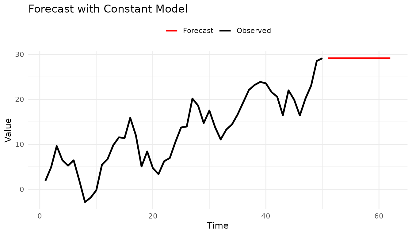
Probabilistic Forecasting
Most real-world forecasts need uncertainty quantification. Let’s add prediction intervals.
Empirical Intervals
The empirical method generates prediction intervals by bootstrapping from residuals:
# Forecast with prediction intervals
fc_with_intervals <- forecast(
  fitted,
  interval_method = EmpiricalInterval(
    n_trajectories = 1000,
    seed = 42
  ),
  horizon = 1:12,
  levels = c(0.50, 0.90, 0.95),
  include_median = FALSE,
  model_name = "Constant"
)

# Convert to hubverse format for visualization
constant_hubverse <- as_hubverse(
  fc_with_intervals,
  start_date = as.Date("2024-01-01"),
  horizon_unit = "week",
  observed_data = full_data
)

# Visualize with hubVis
library(hubVis)
hubVis::plot_step_ahead_model_output(
  constant_hubverse$model_output,
  constant_hubverse$target_data,
  intervals = c(0.5, 0.9, 0.95),
  interactive = TRUE
)
#> Warning: ! `model_out_tbl` must be a `model_out_tbl`. Class
#> applied by default
Try a More Advanced Model
Let’s use an ARMA model for better forecasting:
# Create ARMA(2,1) model
arma_model <- ARMAModel(p = 2, q = 1)

# Fit and forecast with prediction intervals
arma_fitted <- fit_baseline(data, arma_model)
arma_fc <- forecast(
  arma_fitted,
  interval_method = EmpiricalInterval(n_trajectories = 1000),
  horizon = 1:12,
  levels = c(0.50, 0.90, 0.95),
  include_median = FALSE,
  model_name = "ARMA(2,1)"
)

# Convert to hubverse format for visualization
arma_hubverse <- as_hubverse(
  arma_fc,
  start_date = as.Date("2024-01-01"),
  horizon_unit = "week",
  observed_data = full_data
)

# Visualize with hubVis
hubVis::plot_step_ahead_model_output(
  arma_hubverse$model_output,
  arma_hubverse$target_data,
  intervals = c(0.5, 0.9, 0.95),
  interactive = TRUE
)
#> Warning: ! `model_out_tbl` must be a `model_out_tbl`. Class
#> applied by default
The hubVis visualizations show:
- Prediction intervals at 50%, 90%, and 95% confidence levels
- Observed truth values overlaid on the forecasts
Model Evaluation
This package integrates seamlessly with scoringutils for forecast evaluation using proper scoring rules.
For probabilistic forecasts with prediction intervals, use WIS (Weighted Interval Score) and interval coverage:
Compare Multiple Models
For probabilistic forecasts, use proper scoring rules like WIS (Weighted Interval Score):
# Create multiple models
models <- list(
  Constant = ConstantModel(),
  ARMA = ARMAModel(p = 1, q = 1),
  Marginal = MarginalModel()
)

# Fit each model with prediction intervals
forecasts <- lapply(names(models), function(name) {
  fitted <- fit_baseline(data, models[[name]])
  forecast(fitted,
    interval_method = EmpiricalInterval(n_trajectories = 1000),
    horizon = 1:12,
    levels = c(0.50, 0.90, 0.95),
    include_median = FALSE,
    model_name = name
  )
})

# Combine all forecasts for comparison
all_quantiles <- do.call(rbind, lapply(forecasts, function(fc) {
  scoringutils::as_forecast_quantile(add_truth(fc, truth))
}))

# Re-validate as forecast object after rbind
all_quantiles <- scoringutils::as_forecast_quantile(all_quantiles)

# Score all models
scores <- scoringutils::score(all_quantiles)
#> ℹ Median not available, interpolating median from the two innermost quantiles
#>   in order to compute bias.
#> Warning: ! Computation for `interval_coverage_90` failed. Error: ! To compute the
#>   interval coverage for an interval range of "90%", the 0.05 and 0.95 quantiles
#>   are required.
#> Warning: ! Computation for `ae_median` failed. Error: ! In order to compute the absolute
#>   error of the median, "0.5" must be among the quantiles given.
score_summary <- scoringutils::summarise_scores(scores, by = "model")

# Display key metrics
comparison <- data.frame(
  Model = score_summary$model,
  WIS = round(score_summary$wis, 2),
  Coverage_50 = paste0(round(score_summary$interval_coverage_50 * 100, 1), "%"),
  Coverage_90 = paste0(round(score_summary$interval_coverage_90 * 100, 1), "%"),
  Coverage_95 = paste0(round(score_summary$interval_coverage_95 * 100, 1), "%")
)
print(comparison)
#>      Model  WIS Coverage_50 Coverage_90 Coverage_95
#> 1 Constant 1.32         50%           %           %
#> 2     ARMA 1.33       41.7%           %           %
#> 3 Marginal 4.14        8.3%           %           %

cat("\nBest model by WIS:", comparison$Model[which.min(score_summary$wis)], "\n")
#>
#> Best model by WIS: Constant

# Visualize model comparison with hubVis
comparison_hubverse <- as_hubverse(
  all_quantiles,
  start_date = as.Date("2024-01-01"),
  horizon_unit = "week",
  observed_data = full_data
)

hubVis::plot_step_ahead_model_output(
  comparison_hubverse$model_output,
  comparison_hubverse$target_data,
  intervals = c(0.5, 0.9, 0.95),
  interactive = TRUE
)
#> Warning: ! `model_out_tbl` must be a `model_out_tbl`. Class
#> applied by default
Working with Seasonal Data
For data with strong seasonal patterns, use seasonal models:
# Generate seasonal data: 15 years training (Jan 2010-Dec 2024) + 1 year test (2025)
set.seed(789)
n_total_months <- 192  # 16 years total
n_train_months <- 180  # 15 years for training
full_seasonal <- 10 + 5 * sin(2 * pi * (1:n_total_months) / 12) + rnorm(n_total_months, sd = 0.5)
seasonal_data <- full_seasonal[1:n_train_months]
future_seasonal <- full_seasonal[(n_train_months + 1):n_total_months]

# STL decomposition model
stl_model <- STLModel(s = 12)
stl_fitted <- fit_baseline(seasonal_data, stl_model)

stl_fc <- forecast(stl_fitted,
  interval_method = EmpiricalInterval(n_trajectories = 1000),
  horizon = 1:12,
  levels = c(0.50, 0.90, 0.95),
  include_median = FALSE,
  truth = future_seasonal,
  model_name = "STL"
)

# Last Similar Dates model
lsd_model <- LSDModel(window_width = 10, s = 12)
lsd_fitted <- fit_baseline(seasonal_data, lsd_model)
lsd_fc <- forecast(lsd_fitted,
  interval_method = EmpiricalInterval(n_trajectories = 1000),
  horizon = 1:12,
  levels = c(0.50, 0.90, 0.95),
  include_median = FALSE,
  truth = future_seasonal,
  model_name = "LSD"
)

# Combine forecasts for hubVis visualization
stl_quantile <- scoringutils::as_forecast_quantile(stl_fc)
lsd_quantile <- scoringutils::as_forecast_quantile(lsd_fc)
combined_quantile <- rbind(stl_quantile, lsd_quantile)

# Convert to hubverse format (data from Jan 2010 to Dec 2025)
seasonal_hubverse <- as_hubverse(
  combined_quantile,
  start_date = as.Date("2010-01-01"),
  horizon_unit = "month",
  observed_data = full_seasonal
)

# Filter to show only last 5 years + forecast for cleaner visualization
cutoff_date <- as.Date("2020-01-01")
filtered_target <- seasonal_hubverse$target_data[seasonal_hubverse$target_data$date >= cutoff_date, ]
filtered_output <- seasonal_hubverse$model_output[seasonal_hubverse$model_output$target_date >= cutoff_date, ]

# Visualize both models with hubVis
hubVis::plot_step_ahead_model_output(
  filtered_output,
  filtered_target,
  intervals = c(0.5, 0.9, 0.95),
  interactive = TRUE
)
#> Warning: ! `model_out_tbl` must be a `model_out_tbl`. Class
#> applied by default
Data Transformations
For data with non-constant variance or non-negativity constraints, use transformations.
# Example: exponential growth (log transform stabilizes variance)
data_exp <- exp(rnorm(50, mean = 2, sd = 0.3))

# 1. Transform data
log_data <- log(data_exp)

# 2. Fit model on transformed scale
model <- ConstantModel()
fitted <- fit_baseline(log_data, model)

# 3. Forecast on transformed scale
fc <- forecast(fitted,
  interval_method = NoInterval(),
  horizon = 1:12
)

# 4. Back-transform to original scale
fc$mean <- exp(fc$mean)

# Now fc$mean is in the original scale
print(fc$mean)
#>  [1] 5.863768 5.863768 5.863768 5.863768 5.863768 5.863768 5.863768 5.863768
#>  [9] 5.863768 5.863768 5.863768 5.863768
See vignette("transformations") for detailed guidance on
transformations.
Utility Functions
forecastbaselines provides helpful utilities for working with forecast objects:
# Check what components are available
has_mean(fc) # TRUE
#> [1] TRUE
has_median(fc) # FALSE (not requested)
#> [1] TRUE
has_truth(fc) # FALSE (not provided)
#> [1] FALSE

# Add components
median_vals <- fc$mean # For demo, use mean as median
fc_with_median <- add_median(fc, median_vals)
has_median(fc_with_median) # TRUE
#> [1] TRUE

# Add truth values for scoring
fc_with_truth <- add_truth(fc, truth)
has_truth(fc_with_truth) # TRUE
#> [1] TRUE

# Filter/subset forecasts
fc_short <- truncate_horizon(fc, max_h = 5)
fc_selected <- filter_horizons(fc, horizons = c(1, 3, 6, 12))
Next Steps
Now that you’ve learned the basics, explore:
vignette("forecast-models")- Detailed guide to all 10 models, when to use each, and their parametersvignette("transformations")- Guide to data transformations with examplesPackage documentation - Run
?forecastbaselinesorhelp(package = "forecastbaselines")Examples - Check the
examples/directory in the package for complete workflows
Quick Reference
Basic Workflow
# 1. Setup (once)
setup_ForecastBaselines()

# 2. Create model
model <- ARMAModel(p = 2, q = 1)

# 3. Fit to data
fitted <- fit_baseline(data, model)

# 4. Generate forecasts
fc <- forecast(fitted,
  interval_method = EmpiricalInterval(n_trajectories = 1000),
  horizon = 1:12,
  levels = 0.95,
  truth = truth_values,
  model_name = "ARMA(2,1)"
)

# 5. Score forecasts
fc_point <- scoringutils::as_forecast_point(fc)
scores <- scoringutils::score(fc_point)
scores_summary <- scoringutils::summarise_scores(scores, by = "model")
mae <- scores_summary$ae_point
Common Models
# Simple
ConstantModel() # Naive forecast
MarginalModel() # Sample from marginal distribution

# Seasonal
STLModel(s = 12) # Monthly seasonality
LSDModel(window_width = 10, s = 12) # Last similar dates

# Time Series
ARMAModel(p = 2, q = 1) # ARMA
ETSModel() # Exponential smoothingTroubleshooting
Julia not found:
# Specify Julia path manually
Sys.setenv(JULIA_HOME = "/path/to/julia/bin")
setup_ForecastBaselines()
Package not loading:
# Check if Julia is set up
is_setup() # Should return TRUE

# Re-run setup if needed
setup_ForecastBaselines()
Getting errors during forecasting:
# Check your data
summary(data) # No NAs or infinite values?
length(data) # Enough observations?

# Check model parameters
# e.g., ARMA needs p + q < length(data)
For more help, see the GitHub Issues.