Getting started with {ringbp} • ringbp

Introduction

Understanding how an infectious disease might spread, and under what conditions it can be controlled, is crucial for public health planning. The {ringbp} R package provides tools for simulating infectious disease transmission using a branching process model with explicit representation of case detection, isolation, and contact tracing. The package was developed in the early phase of the COVID-19 pandemic to support epidemiological analyses of outbreak dynamics and control feasibility.

This vignette provides a brief introduction to the package and demonstrates how to:

load ringbp
specify epidemiological parameters
run outbreak simulations
plot and summarise simulation results

It concludes with a simplified version of the analysis of COVID-19 control feasibility from Hellewell et al. (2020).

Firstly, we load the {ringbp} package, as well as the {data.table} and {tinyplot} packages which are used in this vignette.

library(ringbp)
library(data.table)
library(tinyplot)

Model overview

At its core, {ringbp} simulates outbreaks using a branching process model. Each infected individual generates secondary infections according to an offspring distribution, with modifications arising from:

delays between infection, symptom onset, and isolation
probabilities governing asymptomatic infection and case detection
optional intervention mechanisms such as quarantine

Simulations are constructed by combining a set of options that describe these components and then running one or more stochastic outbreak realisations.

For a more detailed exposition of the {ringbp} epidemiological model and how non-pharmaceutical interventions influence disease transmission see the ringbp-model.Rmd vignette.

Specifying model components

Offspring distributions

The offspring distribution is a discrete probability distribution that describes the random number of secondary infections (offspring/descendants) generated by a single infected individual during their entire infectious period.

The mean of the offspring distribution is the basic reproduction number ( $R_0$ ), which is defined as the average number of secondary cases caused by one infected individual in a fully susceptible population. The model assumes that an infinite supply of susceptibles is always available to infect, making it suitable for modelling of early outbreaks of pathogens that have not previously spread in a population.

The number of secondary infections is defined using offspring_opts(). Different distributions can be specified for individuals in the community (community), those who are isolated (isolated) and infected individuals that are asymptomatic (or paucisymptomatic) (asymptomatic).

offspring <- offspring_opts(
  community = \(n) rnbinom(n = n, mu = 2.5, size = 0.16),
  isolated = \(n) rgeom(n = n, prob = 0.8), 
  asymptomatic = \(n) rpois(n = n, lambda = 1.5)
)

The offspring distribution for asymptomatic individuals (asymptomatic) does not need to be specified, in which case it is assumed to be the same as the offspring distribution of symptomatic infectors in the community (community).

Delay distributions

Key epidemiological delays, such as the incubation period (incubation_period) and time from symptom onset to isolation (onset_to_isolation), are specified using delay_opts().

delays <- delay_opts(
  incubation_period = \(n) rlnorm(n, meanlog = 0.9, sdlog = 0.5),
  onset_to_isolation = \(n) rgamma(n, shape = 3, scale = 2)
)

Isolation is the separation of infectious individuals from others, with the aim to prevent further transmission.

In the {ringbp} model, isolated individuals have their own transmission dynamics (see offspring_opts() above). {ringbp} allows infected individuals in isolation to transmit (i.e. non-zero reproduction number), and can even have higher transmissibility than infectors in the community.

The arguments to both offspring_opts() and delay_opts() are functions of n: they take an integer n and return a vector of n random samples from a given distribution. This lets you sample offspring or delay values for multiple individuals in a single step of the simulation.

Event probabilities

Probabilities governing infection and detection events are set using event_prob_opts(). The probability that an infector is asymptomatic (asymptomatic), the proportion of disease transmission that occurs before symptom onset (presymptomatic_transmission), and the proportion of symptomatic individuals that are ascertained by contact tracing (symptomatic_ascertained).

event_probs <- event_prob_opts(
  asymptomatic = 0.1,
  presymptomatic_transmission = 0.5,
  symptomatic_ascertained = 0.2
)

Contact tracing is the process of identifying and isolating people who have been in contact with individuals that have tested positive for the infection.

Intervention options

Quarantine in the {ringbp} model is defined as the isolation of individuals independent of their infection status. Contacts can be isolated before they are symptomatic once the infecting individual is confirmed to be infected and goes into isolation. It differs from isolation in the model, which requires the infectee to be symptomatic.

Interventions, thus far only quarantine (quarantine) is implemented, can be turned on or off via intervention_opts().

interventions <- intervention_opts(quarantine = FALSE)

By default, isolation of symptomatic cases is active and qurantine is not active.

Simulation controls

Finally, global simulation limits (for example, maximum duration (cap_max_days) or outbreak size (cap_cases)) are specified using sim_opts().

sim <- sim_opts(
  cap_max_days = 350,
  cap_cases = 4500
)

Running outbreak simulations

With all components defined, simulations can be run using scenario_sim(). The example below runs 100 independent outbreak simulations starting from a single initial case.

Stochastic epidemic model: the {ringbp} model uses random simulations to reflect the inherent uncertainty in real‑world outbreaks.

We set the seed to ensure we have the same output each time the vignette is rendered. When using {ringbp}, setting the seed is not required unless you need to simulate the same outbreak multiple times.

set.seed(1)

outbreak <- scenario_sim(
  n = 100,
  initial_cases = 1,
  offspring = offspring,
  delays = delays,
  event_probs = event_probs,
  interventions = interventions,
  sim = sim
)

The returned object is a data.table containing the simulated outbreak trajectories. The columns are:

sim: simulation replicate ID
week: outbreak week, zero indexed
weekly_cases: number of new cases that week
cumulative: cumulative weekly cases
effective_r0: the effective reproduction number, the same for each simulation replicate
cases_per_gen: the number of cases per generation of the outbreak

Visualising results

A simple way to explore results is to plot cumulative cases over time.

tinyplot(
  cumulative ~ week | as.factor(sim), 
  data = outbreak, 
  type = "l", 
  lwd = 3,
  ylab = "Cumulative number of cases", 
  xlab = "Week",
  legend = FALSE,
  theme = "clean"
)

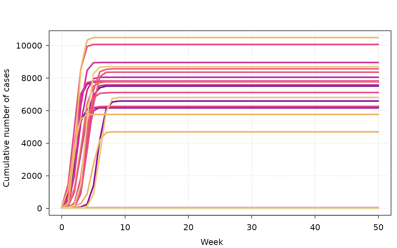
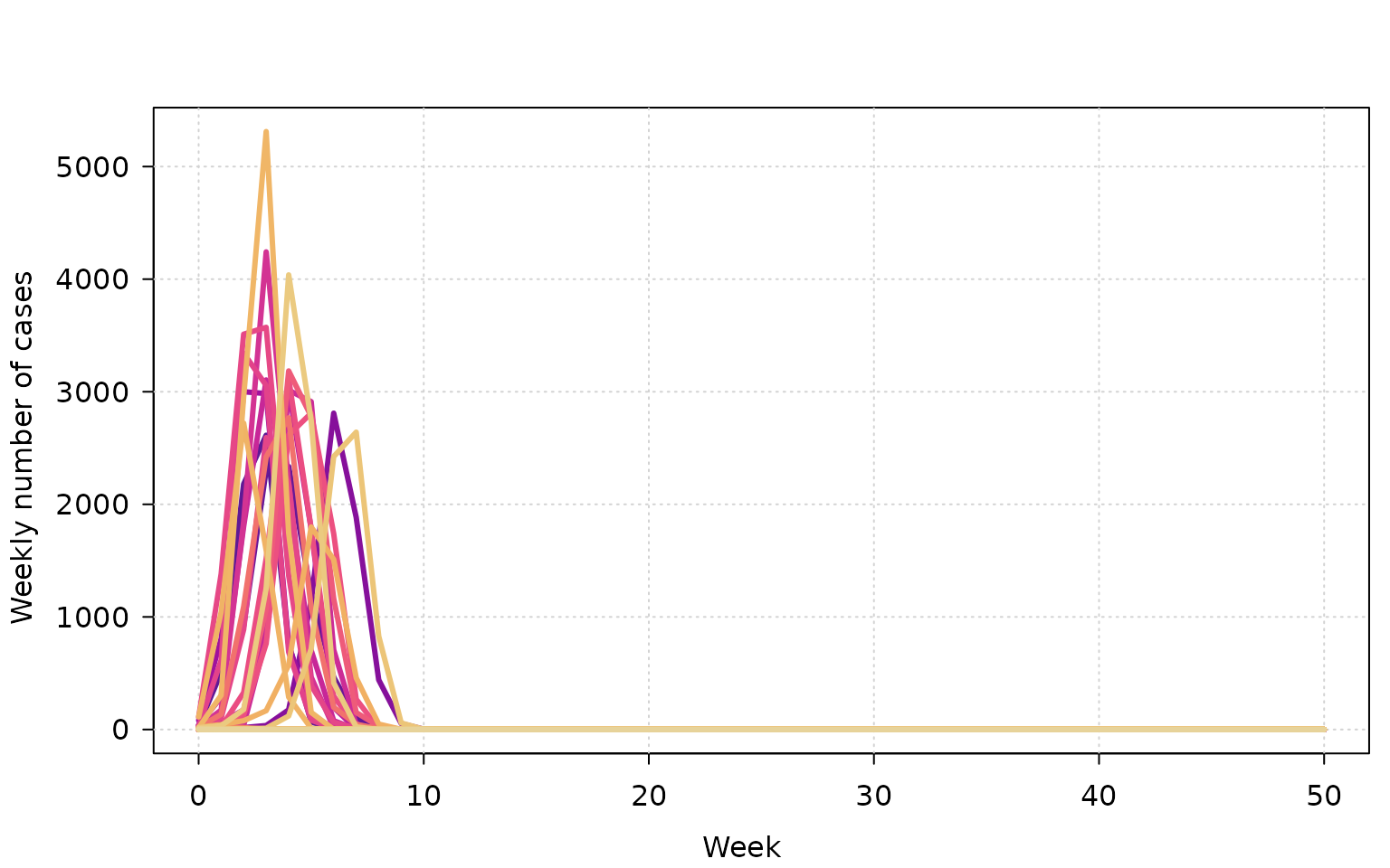
We can also plot the weekly incidence of cases. Note: the maximum number of cases in the simulation is set to 4,500, so the decline in cases to zero is due to reaching that upper bound.

tinyplot(
  weekly_cases ~ week | as.factor(sim), 
  data = outbreak, 
  type = "l", 
  lwd = 3,
  ylab = "Weekly number of cases", 
  xlab = "Week",
  legend = FALSE,
  theme = "clean"
)

Summarising outcomes

A common quantity of interest is the probability that an outbreak goes extinct (i.e. dies out without sustained transmission). This can be calculated using extinct_prob().

extinct_prob(outbreak)
#> Calculating extinction using the extinction status from the simulation.
#> [1] 0.8

By default, extinction is defined as all infectious individuals have had the opportunity to transmit but no new infections are generated. The extinction_week argument in extinct_prob() can also be used to specify whether extinction has happened by a certain week, e.g. extinct_prob(..., extinction_week = 5) checks whether extinction has occurred by week 5 of the outbreak. See ?extinct_prob for other methods of checking for extinction.

Simplified COVID-19 contact tracing effectiveness analysis

Next we demonstrate how to use {ringbp} to reproduce a simplified version of the outbreak control analysis from Hellewell et al. (2020). This study, published in the first months of the COVID-19 pandemic, modelled the probability that an introduced COVID-19 outbreak is contained by isolation and contact tracing. Containment was defined as no disease transmission between weeks 12-16 of the outbreak and the outbreak not reaching 5,000 total cases.

Using the functions described above we define several parameter sets to analyse how varying the basic reproduction number in the community, the proportion of contacts successfully traced, and the number of initial infectors that seed independent outbreaks influence the likelihood of outbreak control.

This is a simplified version of the analysis from Hellewell et al. (2020), for the full analysis see the GitHub repository with the analysis scripts.

Define epidemiological parameters

scenarios <- data.table(
  expand.grid(
    initial_cases = c(5, 20),
    r0_community = c(1.5, 2.5),
    symptomatic_ascertained = c(0, 0.5, 1)
  )
)
scenarios[, scenario :=  1:.N]
scenarios <- scenarios[, list(data = list(.SD)), by = scenario]

Run the simulation

n <- 10

scenarios[, sims := lapply(data, \(x, n) {
  scenario_sim(
    n = n,
    initial_cases = x$initial_cases,
    offspring = offspring_opts(
      community = \(n) rnbinom(n = n, mu = x$r0_community, size = 0.16),
      isolated = \(n) rnbinom(n = n, mu = 0, size = 1)
    ),
    delays = delay_opts(
      incubation_period = \(n) rweibull(n, shape = 1.65, scale = 4.28),
      onset_to_isolation = \(n) rweibull(n, shape = 1.65, scale = 2.31)
    ),
    event_probs = event_prob_opts(
       asymptomatic = 0.1,
       presymptomatic_transmission = 0.1,
       symptomatic_ascertained = x$symptomatic_ascertained
    ),
    interventions = intervention_opts(quarantine = FALSE),
    sim = sim_opts(cap_max_days = 365, cap_cases = 5000)
  )
  },
  n = n
)]

For a more detailed example of running {ringbp} across multiple parameter sets see the parameter-sweep.Rmd vignette, which also includes information on how to parallelise the simulation.


scenarios[, 
  pext := extinct_prob(sims[[1]], extinction_week = 12:16), 
  by = scenario
]
#> Calculating extinction as no new cases within weeks: 12 to 16 (inclusive).
#> Calculating extinction as no new cases within weeks: 12 to 16 (inclusive).
#> Calculating extinction as no new cases within weeks: 12 to 16 (inclusive).
#> Calculating extinction as no new cases within weeks: 12 to 16 (inclusive).
#> Calculating extinction as no new cases within weeks: 12 to 16 (inclusive).
#> Calculating extinction as no new cases within weeks: 12 to 16 (inclusive).
#> Calculating extinction as no new cases within weeks: 12 to 16 (inclusive).
#> Calculating extinction as no new cases within weeks: 12 to 16 (inclusive).
#> Calculating extinction as no new cases within weeks: 12 to 16 (inclusive).
#> Calculating extinction as no new cases within weeks: 12 to 16 (inclusive).
#> Calculating extinction as no new cases within weeks: 12 to 16 (inclusive).
#> Calculating extinction as no new cases within weeks: 12 to 16 (inclusive).

# probability of extinction for each scenario
scenarios$pext
#>  [1] 0.9 0.5 0.5 0.2 1.0 1.0 0.9 0.5 1.0 1.0 1.0 0.9

Hellewell et al. (2020) used {ringbp} to show that:

Outbreaks are controllable if contact tracing is fast and covers a high proportion of contacts
Delays in isolating cases or many undetected asymptomatic cases make control unlikely
Small initial clusters are easier to contain than larger ones

{ringbp} Use Cases

This vignette has focused on the high-level workflow for running simulations with {ringbp}. Further uses of the package include, but are not limited to:

Simulate outbreaks under different assumptions about $R_0$ , incubation period, and proportion of asymptomatic infections.
Explore the impact of delays in isolation and the effectiveness of contact tracing.
Estimate the probability of outbreak extinction under different intervention strategies.

References

Hellewell, Joel, Sam Abbott, Amy Gimma, Nikos I Bosse, Christopher I Jarvis, Timothy W Russell, James D Munday, et al. 2020. “Feasibility of Controlling COVID-19 Outbreaks by Isolation of Cases and Contacts.” The Lancet Global Health 8 (4): e488–96. https://doi.org/10.1016/s2214-109x(20)30074-7.