Intervention-aware R(t) walkthrough

The base joint_model fits R(t) as an unconstrained weekly random walk. Outbreaks with a known intervention may invite stronger structure: a break point, or a random walk plus a one-sided shock that can only drop R after the intervention date. This page compares three intervention-aware variants on the same real-time cut-off — the 18-case wave at Date("2018-12-31") — holding everything else constant.

All three scenarios are fit-side assumptions about R(t). They are not claims about what happened in Epuyén; they describe what the data imply if we constrain R(t) to behave a particular way around the assumed intervention date.

julia

using TransmissionLinelist
using AlgebraOfGraphics: data, mapping, visual, draw
using DataFrames: DataFrame, groupby, nrow
using DataFramesMeta: @chain, @rtransform, @rsubset, @select, @transform,
                      @combine, @subset
using Dates: Dates, Date, Day
using Distributions: Distributions, Normal, LogNormal, NegativeBinomial,
                     truncated, logpdf, cdf
using Random
using Statistics: quantile, mean, var
using CairoMakie
using CairoMakie: Band, Lines, Hist
using FlexiChains: FlexiChains
using Turing: Turing, @model, to_submodel, DynamicPPL
using Logging: Logging

Random.seed!(20260512)
# Silence the NUTS "Found initial step size" Info logs.
Logging.disable_logging(Logging.Info)

LogLevel(1)

Setup

Load the closed-out line list and build the model inputs and weekly knot grid. The intervention timing is a model-side argument, not a data cut-off — the fits see the full outbreak.

julia

intervention_date = Date("2018-12-31")
ll = load_linelist();
t0_ref = minimum(ll.onset_date) - Day(60)
d = build_data(ll; t0 = t0_ref)
edges = prepare_rt_edges(t0_ref)
intervention_day = Float64(Dates.value(intervention_date - t0_ref))
seed = 20260512

20260512

Submodel variants

Two new R(t) submodels are defined inline for this page. Both return (; log_R) so the joint model's case_model consumes them unchanged. log_R is registered on the chain via := so downstream summaries (vector_chain(chn, :log_R), rt_band, …) keep working.

Two-level step (intervention-only)

A single break point at intervention_day: one log-R before, one after. Each knot's log-R is set to one of the two scalars depending on which side of the break point it falls.

julia

@model function step_rt_submodel(edges, intervention_day::Real;
        pre_prior = Normal(log(1.5), 1.0),
        post_prior = Normal(log(1.0), 1.0))
    log_R_pre ~ pre_prior
    log_R_post ~ post_prior
    log_R := [e < intervention_day ? log_R_pre : log_R_post for e in edges]
    return (; log_R)
end

step_rt_submodel (generic function with 2 methods)

Random walk plus one-sided post-intervention shock

Standard random walk plus a multiplicative exp(shock) applied at every knot on or after intervention_day. The shock prior is truncated above at zero so the model can only express a drop in R after the intervention.

julia

@model function rw_plus_shock_rt_submodel(edges, intervention_day::Real;
        init_prior = Normal(log(1.5), 1.0),
        sigma_prior = truncated(Normal(0.0, 0.2); lower = 0),
        shock_prior = truncated(Normal(0.0, 0.5); upper = 0))
    n_knots = length(edges)
    σ_rw ~ sigma_prior
    log_R_init ~ init_prior
    shock ~ shock_prior
    T = typeof(log_R_init)
    ε ~ Turing.filldist(Normal(zero(T), one(T)), n_knots - 1)
    base = vcat(log_R_init, log_R_init .+ accumulate(+, σ_rw .* ε))
    log_R := [base[i] + (edges[i] >= intervention_day ? shock : zero(T))
              for i in 1:n_knots]
    return (; log_R)
end

rw_plus_shock_rt_submodel (generic function with 2 methods)

Fits

Three joint fits on the same real-time view, identical seed, differing only in the R(t) submodel.

julia

m_rw = joint_model(d, edges)
m_step = joint_model(d, edges;
    rt = step_rt_submodel(edges, intervention_day))
m_shock = joint_model(d, edges;
    rt = rw_plus_shock_rt_submodel(edges, intervention_day))

chn_rw = sample_fit(m_rw; seed = seed)
chn_step = sample_fit(m_step; seed = seed)
chn_shock = sample_fit(m_shock; seed = seed)

post_rw = summarise(chn_rw)
post_step = summarise(chn_step)
post_shock = summarise(chn_shock)

(μ_inc = [3.152882869869638, 3.0054115480109727, 3.0877253625775114, 3.1224091539106262, 3.110633732141487, 3.1832764017024506, 2.9200981116181173, 2.891276170353263, 2.865818177369781, 3.225361885031595  …  3.0732414517637863, 3.070443812401704, 3.052486134588899, 3.075093053872934, 2.963312385670861, 3.053738948832992, 3.0141669403994493, 3.0921505596123984, 3.0931141739045938, 3.0183730659813444], σ_inc = [0.31409191463916486, 0.3206859669637448, 0.2664924395356561, 0.39212330104357923, 0.25128724570915206, 0.28699777583620145, 0.35330322278176995, 0.41871903889443496, 0.3907983290236691, 0.3100578715735163  …  0.27469782529569053, 0.3478881161559974, 0.25118892134297977, 0.3639707573783475, 0.35270719233941505, 0.3626858780129023, 0.3394938406871281, 0.30118775059701003, 0.31501577413192744, 0.2854501566991917], μ_δ = [0.09278003111191474, 0.06330172096057916, 0.483211012883984, 0.13299420206275744, 0.25706438368956835, 0.019302489792137553, 0.04629319118070987, 0.3926278308810662, 0.09959763513831245, 0.18429400779294808  …  0.40200855427134763, 0.2071753270948008, 0.09243655355797326, 0.33731216820683363, 0.04963063605550838, 0.23918034071076275, 0.246843777767363, 0.30934356404430513, 0.25521502594304385, 0.07701882453749495], σ_δ = [0.5511713259496638, 0.6990662988742412, 0.7250499628553858, 0.6302114490731218, 0.6189606273073042, 0.618691339790974, 0.5801199317645234, 0.6218589288270814, 0.5788334765460044, 0.5908874109508805  …  0.5282033258165658, 0.6868332558752249, 0.699873348860637, 0.666790173369599, 0.630676018150835, 0.6318895111893941, 0.6611021700891707, 0.6387437406624253, 0.5904413984962685, 0.6651435179117765], k = [0.3187544910422385, 0.5225040492788288, 0.20271952505953764, 0.8386798782013019, 0.3202405164948406, 0.42661537722756626, 0.2668067038458164, 0.264846201262873, 0.1873292339344069, 0.46298121338697634  …  0.4448880088098612, 0.2891262646192541, 0.35819013197590777, 0.333566637305009, 0.7209210278915316, 0.36901597520188056, 0.41436412915803505, 0.16484657469947975, 0.12528690417325497, 0.4158321163798924], σ_rw = [0.12884105331354317, 0.0320706884312439, 0.060744056431785445, 0.20802870759987674, 0.2751649749355067, 0.24116437349687767, 0.05325092829211772, 0.10015984615768132, 0.11459880543693775, 0.08099148557928716  …  0.7500108433143424, 0.03411517639883906, 0.2965096080124824, 0.3293767958240434, 0.18791389775792858, 0.1119912177138856, 0.1692646999782373, 0.08004693369569331, 0.14440983641083116, 0.27302856097979034], log_R_chain = [[-0.4681231181517373, 0.3391805260692611, 0.07019985712267787, 0.4463975902209093, 0.605137442176313, 0.4248011049003154, 0.4933384711150656, 0.29029150000615217, 0.3269948716761712, 0.4033247114152443  …  1.4464843938227017, 0.41635141640355355, 0.6601268179143494, 0.3387307518986521, 0.40016335773515554, -0.412324055771114, 0.009505852261786296, 0.9784761948958365, 0.7431193259689987, 0.4221959030939505], [-0.37573891339377485, 0.3919691862143078, 0.14996198037516884, 0.3120932288584004, 0.3497160563035322, 0.3253987226549204, 0.5069356329211012, 0.21000535750794597, 0.31946825017118113, 0.4172639511007787  …  1.042102429269332, 0.43917841120355705, 0.6684343172025372, 0.5304490265941222, 0.21630077999171846, -0.379589523585107, 0.05985535787238287, 0.8586946179263493, 0.48051502470565743, 0.3385381724351546], [-0.5281586402327838, 0.4667592706356347, 0.160197766526187, 0.3635688278102145, 0.3425765247469832, 0.4617050268918509, 0.5207775639089908, 0.2182964072823771, 0.10485544641222652, 0.5665681648631361  …  1.732061046597609, 0.41263198569478526, 0.6192098232499277, 0.45856745205876626, 0.22756983540236125, -0.49181419864916315, -0.07012243694344507, 0.9263163007740486, 0.6563862997022051, 0.07893594183887931], [-0.6490257118789329, 0.4957579371506509, 0.11649325909244211, 0.18973431314908662, 0.1540925162625808, -0.022434229776125747, 0.5513357254952322, 0.39640828649499793, 0.14316013515090348, 0.5987641721130909  …  1.832362030240667, 0.42434730339161975, 0.4479834093056042, 0.37156160615671757, 0.23596409184381423, -0.2763374946720709, 0.22255269471079703, 0.7910223283369002, 0.40801579989156866, 0.011513577051775636], [-0.5332441844252712, 0.5296828420020327, 0.18253785424017877, 0.09217750136371705, 0.26879477426154075, 0.05328816838689632, 0.49975391064054164, 0.36891924373516594, 0.18373660610558637, 0.5750584491862218  …  1.4167603832020819, 0.45934106812476316, -0.07891034609974323, 0.6547219101153647, 0.04872999973164438, -0.3547363602102106, 0.24613494172645936, 0.8067446554728415, 0.44769848251609934, -0.04518453249145149], [-0.5204467431763025, 0.5602341551164524, 0.24433560248671857, -0.4048837543929541, 0.29024934984162915, -0.0804007130024561, 0.5137067706492682, 0.33284227675731304, 0.08851878910678057, 0.6202380081202276  …  1.3932141814738754, 0.4338822734941819, -0.2948321561455718, 0.48205143299181363, -0.1433573157793413, -0.24872421855604837, 0.39980267963456434, 0.7448574841584166, 0.39442604743689147, -0.18731239678311573], [-0.507570500214842, 0.5865278971773268, 0.24784574132086595, -0.8445333658166089, 0.22402355036088323, -0.27575479090659116, 0.5369937946576077, 0.2456191941424155, 0.08875468012530191, 0.5961533089280147  …  0.7554628606033592, 0.44654408663551937, -0.622954748325347, 0.49980118223556047, -0.3861319610370795, -0.3367703405261401, 0.37052368338029645, 0.7472930366464081, 0.25554216524748663, -0.30236775322482246], [-1.5570682030012526, -0.12172233637511132, -0.9105025229383444, -1.4216247162488052, -0.2509086244680735, -0.7768485815291614, -0.10532872466749821, -0.8912038314248137, -0.33369676644247864, -0.5495450689732533  …  -0.11291271039182088, -0.47135742528490593, -1.2639365459673289, -0.9940927403347589, -1.3016199202561676, -0.8053325414811257, 0.008769734511565264, 0.4328566574317576, -0.17823611984241972, -0.438433519136273], [-1.5155061981504492, -0.0962685024040254, -0.8829886023704985, -1.8473971540087737, -0.22276091708082435, -0.6583564970873098, -0.13107290670968091, -0.9063006674523215, -0.3594908724826952, -0.5657770788376248  …  -1.4911410838250683, -0.4152480282596632, -1.1428793323156956, -0.9520566342721049, -1.322439580407893, -0.8088463157898476, -0.07783112924547197, 0.46184374063810696, -0.06211506366540731, -0.6454371275136316], [-1.3463042254303397, -0.13304883095384523, -0.946198814610588, -1.6798398418525067, -0.6152045168821039, -0.9959871306319829, -0.07008905532752774, -0.9610499168137211, -0.38915665722299625, -0.5538877444989312  …  -2.722716998614862, -0.36345672039614907, -1.1856049390532997, -0.821833352287255, -1.4183762905748563, -0.7172152639951919, 0.07922195840465796, 0.48678038287513703, -0.08607209949827599, -0.3232760102083902], [-1.5498128680917715, -0.12356096103849468, -0.9846345195099395, -1.6277042898356235, -0.42299468011879493, -0.7742226236288655, -0.06321178536430361, -0.7709919122924659, -0.15533310093157382, -0.6637889224294115  …  -3.1059139456459226, -0.36160832751877925, -1.1163363529962507, -1.0886630272891074, -1.2378873142746545, -0.6590973517842503, 0.12265031780088875, 0.5313260652681172, 0.03322730128722634, -0.04062508711996608], [-1.5887855026339466, -0.14879280462345512, -1.068076927254776, -1.3421323631149087, -0.7231372623347772, -0.9833777620823645, -0.018609049645786357, -0.9092249775563788, -0.056457104322951535, -0.7299032680828899  …  -3.1708739000093518, -0.3657187530599125, -0.9628017229106007, -1.3264852896840222, -1.0889451141063275, -0.8265093094401884, -0.0928676185176544, 0.5059923217427436, 0.01852821026630741, -0.4082846963293018], [-1.7180877741397895, -0.1332766402403619, -1.0837232935014183, -1.3463445549712065, -0.5341874567529191, -0.8316409566482517, -0.07225959065592857, -1.026540444524521, -0.19750531987686595, -0.64258393521258  …  -1.9438883825107902, -0.42590241008555363, -0.5189290060191706, -1.6216315475540517, -0.9259041784368778, -0.9574501478462046, -0.2820163722784574, 0.5014993024982222, 0.05603037236163366, -0.08966736736986207]], mean_gi_si = [24.67958056541921, 21.323385056091187, 23.202958342655993, 24.648100117340945, 23.411963246038454, 25.159304003416594, 19.78358230995605, 20.059566526441593, 19.056722522260014, 26.586031626954735  …  22.844832103980693, 23.103053068937797, 21.938791188458787, 23.47193709800377, 20.65421447373901, 22.87445402215177, 21.82744833918245, 23.355697820094136, 23.422279675683452, 21.38568732891322], sd_gi_si = [7.9361149677598375, 7.0317448641123015, 6.2062437055113255, 10.014431646279107, 5.943918914060064, 7.392215340586894, 7.219963683295112, 8.631836707637065, 7.722205985388011, 8.407597666173224  …  6.305308003969434, 8.24106272326661, 5.61902801218987, 8.732542989714927, 7.52584580016122, 8.510502727980466, 7.57166198317897, 7.130380553922392, 7.506102690427265, 6.244124206096447], p_pre = Dict(0.0 => [0.4331608651719664, 0.4639243609957149, 0.25256111066507697, 0.416431509963352, 0.33895521701603215, 0.4875554582255573, 0.46819842222501606, 0.26389681210190624, 0.431692770702379, 0.3775606894095737  …  0.22330262605501758, 0.38146384212222956, 0.4474620435627249, 0.30647236535997596, 0.4686378718472967, 0.35252362538608784, 0.3544320055285075, 0.31408650439236036, 0.33278187292723516, 0.4539083819067587], -1.0 => [0.023703248653189544, 0.0641259914984192, 0.020394556657945418, 0.03610434627155928, 0.02113115644949581, 0.04972624609283634, 0.03564852133209361, 0.012563019705167228, 0.028737647604151213, 0.022520926458929773  …  0.003973690978216282, 0.03940814417346458, 0.05927295828333752, 0.02244964738751687, 0.04802679426865944, 0.02493535716354343, 0.029646959083656634, 0.020188411565436406, 0.01675609975371712, 0.0526991375055923], -2.0 => [7.323826750109635e-5, 0.0015811175103455789, 0.0003075325526826703, 0.0003564503517032554, 0.0001328978119017066, 0.0005495881958295513, 0.00020986098761007903, 5.9654616142295965e-5, 0.0001432050530567047, 0.00010923883532960822  …  2.7142500872274846e-6, 0.0006555171423988683, 0.0013960932452716209, 0.00022803036422044484, 0.0005772387787487347, 0.00019733205270576685, 0.00033861739311568317, 0.0001499154301569334, 6.6850165458046e-5, 0.0008961152096414235]))

Sampler health

R̂ near 1 and zero divergences are the targets across all three fits. Step and RW + shock have one extra scalar each (log_R_post, shock) so a small uptick in runtime_seconds is expected.

julia

diag_df = let
    rows = []
    for (name,
        chn) in (("RW (current)", chn_rw),
        ("step (intervention only)", chn_step),
        ("RW + post-shock", chn_shock))
        push!(rows, merge((; scenario = name),
            first(diagnostics_table(chn))))
    end
    DataFrame(rows)
end

3×5 DataFrame

Row	scenario	rhat_max	ess_min	divergences	runtime_seconds
	String	Float64	Float64	Int64	Float64
1	RW (current)	1.00422	1581.12	0	21.671
2	step (intervention only)	1.00396	2233.02	0	65.9033
3	RW + post-shock	1.00377	2240.94	0	78.3062

R(t) trajectories overlaid

Posterior median R(t) with 80% CrI ribbons for all three scenarios on a single panel. The step fit forces a flat-flat shape; the RW + shock fit lets the random walk move freely up to intervention_day and only allows a downward jump at the cut-off; the plain RW fit imposes no intervention structure.

julia

let
    band_rows = DataFrame[]
    for (name,
        post) in (("RW (current)", post_rw),
        ("step (intervention only)", post_step),
        ("RW + post-shock", post_shock))
        tbl = rt_band(post)
        tbl.scenario .= name
        push!(band_rows, tbl)
    end
    df = reduce(vcat, band_rows)
    band_spec = data(df) *
                mapping(:bin => "Bin index",
                    :lo => "R(t) (80% CrI)", :hi;
                    color = :scenario) *
                visual(Band; alpha = 0.2)
    line_spec = data(df) *
                mapping(:bin => "Bin index",
                    :med => "R(t) (80% CrI)";
                    color = :scenario) *
                visual(Lines; linewidth = 2)
    draw(band_spec + line_spec;
        axis = (; limits = (nothing, (0.0, 4.0))),
        figure = (; size = (900, 500)))
end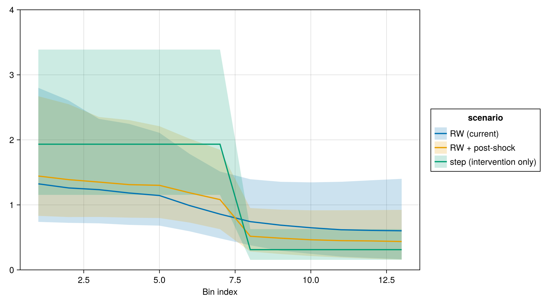

Population marginal posteriors

Overlaid marginals of (μ_inc, σ_inc, μ_δ, σ_δ, k) across the three scenarios. If the population delays move much when only the R(t) half of the likelihood changes, that hints the data carries little information on the delays at this cut-off; otherwise they should overlap.

julia

function plot_marginal_overlay(df; size_kw = (1600, 400))
    spec = data(df) *
           mapping(:value => "value", color = :scenario => "scenario",
               col = :param) *
           visual(Hist; bins = 30, normalization = :pdf, alpha = 0.4)
    return draw(spec;
        facet = (linkxaxes = :colwise, linkyaxes = :none),
        figure = (; size = size_kw))
end

function post_long(post, params; scenario)
    rows = mapreduce(vcat, params) do p
        vals = getproperty(post, p)
        DataFrame(scenario = scenario, param = String(p),
            value = collect(vals))
    end
    return rows
end

let
    params = [:μ_inc, :σ_inc, :μ_δ, :σ_δ, :k]
    df = vcat(
        post_long(post_rw, params; scenario = "RW (current)"),
        post_long(post_step, params;
            scenario = "step (intervention only)"),
        post_long(post_shock, params; scenario = "RW + post-shock"))
    k_cap = @chain df begin
        @rsubset :param == "k" && isfinite(:value)
        quantile(_.value, 0.99)
    end
    df_capped = @rsubset(df, :param != "k" || :value <= k_cap)
    plot_marginal_overlay(df_capped)
end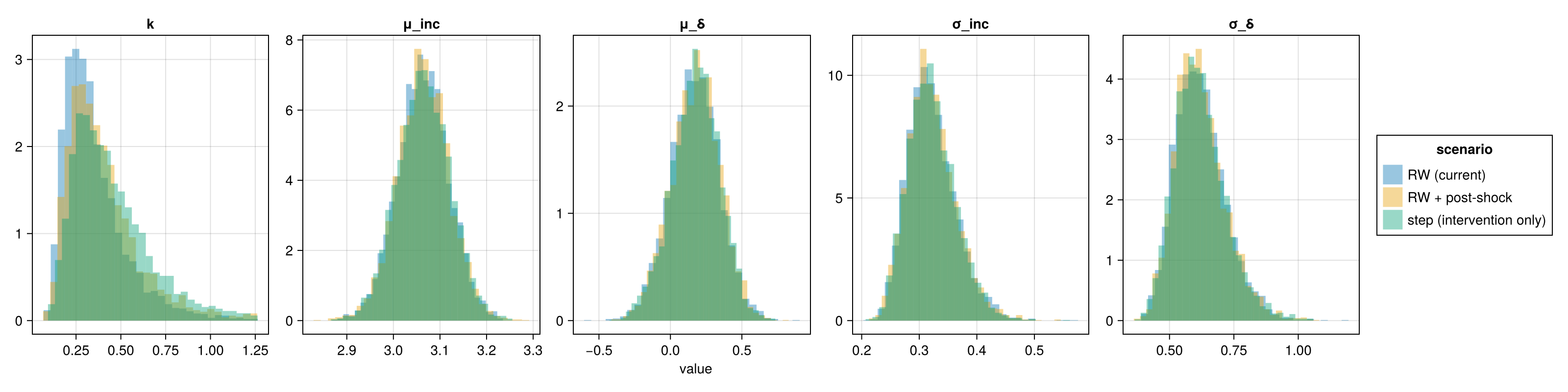

R-pre vs R-post in the intervention-bearing scenarios

For the step model, R-pre and R-post are the two sampled scalars directly. For the RW + post-shock model, R-pre is the exponentiated log-R at the last pre-intervention knot and R-post is R-pre times exp(shock); both pulled from the per-draw :log_R vector to stay consistent with the case_model likelihood.

julia

function effect_size_rows(post; scenario, intervention_idx)
    pre = exp.(post.log_R_chain[intervention_idx - 1])
    post_R = exp.(post.log_R_chain[intervention_idx])
    return DataFrame(
        scenario = scenario,
        median_pre = quantile(pre, 0.5),
        lo_pre = quantile(pre, 0.1),
        hi_pre = quantile(pre, 0.9),
        median_post = quantile(post_R, 0.5),
        lo_post = quantile(post_R, 0.1),
        hi_post = quantile(post_R, 0.9),
        p_drop = mean(post_R .< pre))
end

# Identify the first knot at or after `intervention_day`. With the
# real-time grid the cut-off is the last edge, so this is the final
# knot index.
intervention_idx = findfirst(e -> e >= intervention_day, edges)

effect_df = vcat(
    effect_size_rows(post_step;
        scenario = "step (intervention only)",
        intervention_idx = intervention_idx),
    effect_size_rows(post_shock;
        scenario = "RW + post-shock",
        intervention_idx = intervention_idx))

2×8 DataFrame

Row	scenario	median_pre	lo_pre	hi_pre	median_post	lo_post	hi_post	p_drop
	String	Float64	Float64	Float64	Float64	Float64	Float64	Float64
1	step (intervention only)	1.93297	1.15343	3.38835	0.311251	0.154756	0.627186	0.99525
2	RW + post-shock	1.08111	0.626275	1.84749	0.517168	0.282088	0.950925	0.9815

WAIC comparison on the offspring likelihood

Cheap model comparison: pointwise log-likelihood of the observed offspring count Z_i under each posterior draw, then WAIC = lppd - p_waic summed across cases. Higher (less negative) is better. This conditions on the latent T_onset and log_R per draw, so it is a conditional WAIC over the case-model half of the likelihood — the cleanest cross-scenario comparison given that the R(t) submodel is the only thing changing.

julia

function pointwise_z_loglik(chn, d, edges)
    log_R = vector_chain(chn, :log_R)
    T_onset = vector_chain(chn, :T_onset)
    k_draws = vec(collect(chn[:k]))
    n_draws = length(k_draws)
    N = d.N
    ll = Matrix{Float64}(undef, n_draws, N)
    p_per_source = if d.obs_time !== nothing
        # Reproduce the offspring-completeness thinning so the
        # per-case rate matches the one inside `case_model`.
        μ_inc = vec(collect(chn[:μ_inc]));
        σ_inc = vec(collect(chn[:σ_inc]))
        μ_δ = vec(collect(chn[:μ_δ]));
        σ_δ = vec(collect(chn[:σ_δ]))
        function compute_p(dr, i)
            inc = LogNormal(μ_inc[dr], σ_inc[dr])
            δd = Normal(μ_δ[dr], σ_δ[dr])
            cdf(ConvolvedDelays(inc, δd),
                d.obs_time[i] - T_onset[i][dr])
        end
        compute_p
    else
        (dr, i) -> 1.0
    end
    for dr in 1:n_draws
        logR_d = [log_R[b][dr] for b in eachindex(log_R)]
        for i in 1:N
            R_i = exp(log_R_at(T_onset[i][dr], edges, logR_d))
            p_i = p_per_source(dr, i)
            R_eff = R_i * p_i
            kd = k_draws[dr]
            p = max(kd / (kd + R_eff), eps(typeof(kd)))
            ll[dr, i] = logpdf(NegativeBinomial(kd, p), d.Zobs[i])
        end
    end
    return ll
end

function waic(ll)
    # Standard WAIC: lppd − p_waic, summed across observations.
    lppd = sum(log.(mean(exp.(ll); dims = 1)))
    p_waic = sum(var(ll; dims = 1))
    return (; waic = lppd - p_waic, lppd, p_waic)
end

waic_df = let
    rows = []
    for (name,
        chn) in (("RW (current)", chn_rw),
        ("step (intervention only)", chn_step),
        ("RW + post-shock", chn_shock))
        ll = pointwise_z_loglik(chn, d, edges)
        w = waic(ll)
        push!(rows, (; scenario = name, w...))
    end
    DataFrame(rows)
end

3×4 DataFrame

Row	scenario	waic	lppd	p_waic
	String	Float64	Float64	Float64
1	RW (current)	-40.9585	-38.651	2.30753
2	step (intervention only)	-39.3467	-36.9974	2.34924
3	RW + post-shock	-40.0285	-37.8108	2.2177

Synthesis

The plain RW fit and the RW + post-shock fit both put substantial posterior mass on R(t) below 1 in the final week of the cut-off without requiring an explicit break point, so the data alone are already nudging late R downward. The step fit forces a discrete break, which buys identifiability of R-pre and R-post but cannot represent the gradual rise-and-fall that the RW fit picks out. The RW + post-shock fit nests the plain RW (shock = 0 is at the upper boundary of the shock prior) so its log_R posterior can only move down at the break: if WAIC barely improves over the plain RW, the data are not asking for the extra shock parameter. The R-pre vs R-post tables in effect_df quantify the drop the data attribute to the assumed intervention under each parameterisation; the headline p_drop summarises the posterior probability that R-post is strictly below R-pre.

A fourth scenario varying the right-truncation correction on the delay distributions is discussed in issue #48.

Intervention-aware R(t) walkthrough ​

Setup ​

Submodel variants ​

Two-level step (intervention-only) ​

Random walk plus one-sided post-intervention shock ​

Fits ​

Sampler health ​

R(t) trajectories overlaid ​

Population marginal posteriors ​

R-pre vs R-post in the intervention-bearing scenarios ​

WAIC comparison on the offspring likelihood ​

Synthesis ​

Intervention-aware R(t) walkthrough

Setup

Submodel variants

Two-level step (intervention-only)

Random walk plus one-sided post-intervention shock

Fits

Sampler health

R(t) trajectories overlaid

Population marginal posteriors

R-pre vs R-post in the intervention-bearing scenarios

WAIC comparison on the offspring likelihood

Synthesis