Real-time vs retrospective monitoring
The base joint_model fits a closed-out outbreak with complete observation. In real time, three biases need correcting: 2. Long-incubation cases infected before the cut-off may not yet have developed symptoms — observed incubation periods are enriched for short delays.
Late transmissions from any source may not yet have happened or have not yet been linked — observed transmission timings (δ) are enriched for early / pre-symptomatic events.
Recent source cases have not had time to seed all their offspring — the observed offspring count is a downward-biased estimate of R(t) near the cut-off.
The real-time machinery in joint_model corrects for these via per-case right-truncation on Inc and δ and an offspring-completeness adjustment on the NB offspring count, expressed as the cdf of the ConvolvedDelays distribution δ + Inc(sec). The adjustment is the probability that an offspring's chain has completed by the cut-off, conditional on the source's onset time. The argument is obs_time − T_onset[src], not obs_time − T_inf[src] — the source's own incubation is a sampled latent already scored, so the offspring delay reduces to δ + Inc(sec). This page validates the corrections by fitting the same outbreak at four real-time cut-offs and overlaying the resulting R(t) posteriors and population marginals against a counterfactual retrospective and the full closed-out fit. It also runs a delays-only diagnostic at each cut-off — fitting just the incubation and δ submodels — so that if the full joint fit collapses, we can tell whether the pathology lives in the delay submodels or in the R(t) / case_model half of the likelihood.
Real-time-specific caveats are listed in the Limitations page under the "Real-time fitting caveats" heading.
using TransmissionLinelist
using AlgebraOfGraphics: data, mapping, visual, draw
using DataFrames: DataFrame, groupby, nrow
using DataFramesMeta: @chain, @rtransform, @rsubset, @select, @transform,
                      @combine, @subset
using Dates: Dates, Date, Day
using Random
using Statistics: quantile
using CairoMakie
using CairoMakie: Band, Lines, Hist, VLines
using FlexiChains: FlexiChains
using Turing: DynamicPPL
using Logging: Logging

Random.seed!(20260512)
# Silence the NUTS "Found initial step size" Info logs that would
# otherwise clutter the rendered example output.
Logging.disable_logging(Logging.Info)LogLevel(1)Setup
Four cut-offs are used: 31 December 2018 (about three weeks into the outbreak), 7 January 2019, 14 January 2019, and 21 January 2019. Together they show successive stages of inference as the offspring-completeness window expands: at Dec 31 most late-December sources have had little time to seed offspring; at Jan 7 the completeness factor for those sources has begun to fill in; by Jan 14 the late-December chains have largely played out; and by Jan 21 the early-January chains have also matured, so R(t) at those knots should sharpen toward the retrospective.
obs_dates = [Date("2018-12-31"), Date("2019-01-07"),
    Date("2019-01-14"), Date("2019-01-21")]
ll = load_linelist();
t0_ref = minimum(ll.onset_date) - Day(60)
edges_ref = prepare_rt_edges(t0_ref)
seed = 2026051220260512Data preparation per cut-off
For each obs_date we build two views of the line list:
the counterfactual retrospective (filtered by exposure: cases known to have been infected by
obs_date),the real-time view (filtered by onset: what an analyst sees at
obs_date).
Each cut-off also gets its own weekly knot grid edges_rt truncated at the cut-off so the R(t) posterior does not extend past the observation window.
function prepare_at(ll, obs_date)
    ll_truth = filter_by_exposure(ll, obs_date)
    ll_rt = filter_realtime(ll, obs_date)
    d_truth = build_data(ll_truth; t0 = t0_ref)
    d_rt = build_data(ll_rt; obs_time = obs_date, t0 = t0_ref)
    edges_rt = prepare_rt_edges(t0_ref; obs_time = obs_date)
    return (; obs_date, ll_truth, ll_rt, d_truth, d_rt, edges_rt,
        n_truth = nrow(ll_truth), n_rt = nrow(ll_rt))
end

preps = [prepare_at(ll, obs_date) for obs_date in obs_dates];
Delays-only fits
Fit delays_only_model on both the counterfactual retrospective and the real-time views at each cut-off. These fits drop the R(t) / case_model NB likelihood and condition on only the incubation and δ submodels (plus their truncation in the real-time case). If the delay parameters diverge here, the joint fit at the same cut-off has no chance.
delays_fits = map(preps) do prep
    fit_dly(d) = sample_fit(delays_only_model(d); seed = seed)
    merge(prep, (; chn_dly_truth = fit_dly(prep.d_truth),
        chn_dly_rt = fit_dly(prep.d_rt)))
end;
Delays-only population posteriors per cut-off
Overlaid marginals of (μ_inc, σ_inc, μ_δ, σ_δ) from the delays-only fits at each cut-off, one row per obs_date. If the corrected real-time density tracks the counterfactual retro density on each panel, the right-truncation on Inc and δ alone is enough to recover the population delays from the truncated observations.
The shared marginal-overlay helper plot_marginal_overlay is exported from the package (see src/plots.jl).
Long-form DataFrame of scalar parameter draws from a FlexiChain, selecting on params via FlexiChains' VarName indexing.
function chain_long(chn, params)
    vns = [DynamicPPL.VarName{p}() for p in params]
    @chain DataFrame(FlexiChains.Long(chn[vns])) begin
        @rtransform :param = String(DynamicPPL.getsym(:param))
        @select :iter :chain :param :value
    end
end

delays_marginals_df = let
    params = [:μ_inc, :σ_inc, :μ_δ, :σ_δ]
    @chain delays_fits begin
        map(_) do fit
            t = @transform(chain_long(fit.chn_dly_truth, params),
                :obs_date=string(fit.obs_date),
                :fit="counterfactual retro")
            r = @transform(chain_long(fit.chn_dly_rt, params),
                :obs_date=string(fit.obs_date),
                :fit="corrected real-time")
            vcat(t, r)
        end
        reduce(vcat, _)
    end
end;

plot_marginal_overlay(delays_marginals_df;
    size_kw = (1600, 1300))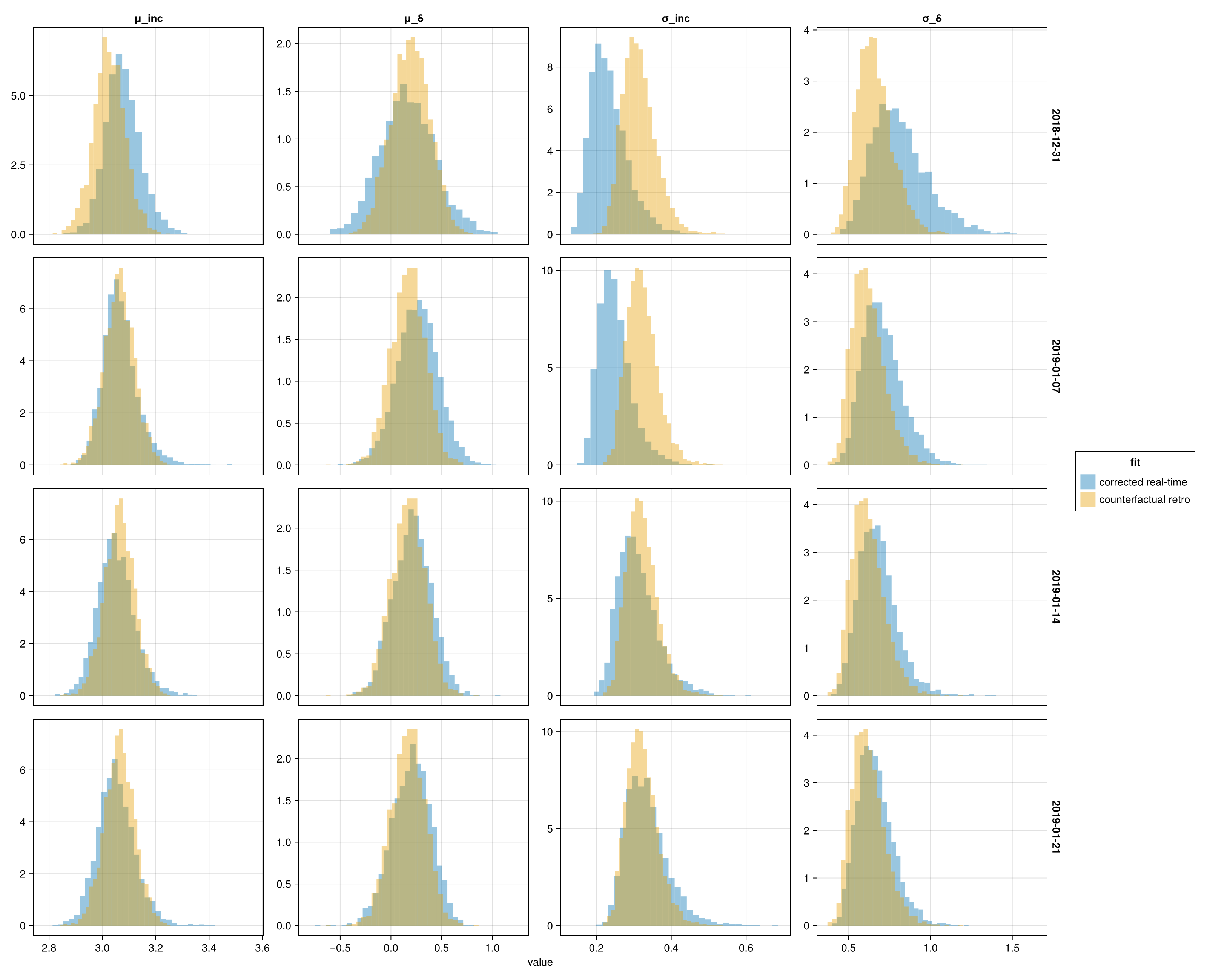
Joint fits
Once the delays-only fits are in hand, fit the full joint model: one full retrospective fit on the closed-out line list (shared comparator across cut-offs) plus, at each cut-off, a counterfactual retro and a corrected real-time joint fit.
The full retrospective fit's standalone diagnostics, headline summary and data plot are not repeated here — see the analysis walkthrough page for those.
d_retro = build_data(ll; t0 = t0_ref);
chn_retro_full = sample_fit(joint_model(d_retro, edges_ref);
    seed = seed);
post_retro_full = summarise(chn_retro_full);

joint_fits = map(delays_fits) do prep
    fit_jnt(d) = sample_fit(joint_model(d, prep.edges_rt); seed = seed)
    chn_truth = fit_jnt(prep.d_truth)
    chn_rt = fit_jnt(prep.d_rt)
    merge(prep,
        (; m_truth = joint_model(prep.d_truth, prep.edges_rt),
            m_rt = joint_model(prep.d_rt, prep.edges_rt),
            chn_truth, chn_rt,
            post_truth = summarise(chn_truth),
            post_rt = summarise(chn_rt)))
end;
Sampler health across all fits
Combined sampler diagnostics with one row per fit — delays-only and joint, retro and real-time, at each cut-off, plus the full retro joint reference. R̂ near 1 and zero divergences are the targets. If R̂ blows up only on the joint rows at a given cut-off, the delay submodels are not to blame and the pathology is in the R(t) / case_model half of the likelihood.
function diag_row(chn, obs_date, fit_kind, n_cases)
    merge((; obs_date, fit_kind, N_cases = n_cases),
        first(diagnostics_table(chn)))
end

diag_df = let
    full = [diag_row(chn_retro_full, missing,
        "full retro (joint)", nrow(ll))]
    per_cut = mapreduce(vcat, zip(delays_fits, joint_fits)) do (dly, jnt)
        [
            diag_row(dly.chn_dly_truth, dly.obs_date,
                "retro (delays only)", dly.n_truth),
            diag_row(dly.chn_dly_rt, dly.obs_date,
                "realtime (delays only)", dly.n_rt),
            diag_row(jnt.chn_truth, jnt.obs_date,
                "retro (joint)", jnt.n_truth),
            diag_row(jnt.chn_rt, jnt.obs_date,
                "realtime (joint)", jnt.n_rt)]
    end
    DataFrame(vcat(full, per_cut))
end| Row | obs_date | fit_kind | N_cases | rhat_max | ess_min | divergences | runtime_seconds |
|---|---|---|---|---|---|---|---|
| Date? | String | Int64 | Float64 | Float64 | Int64 | Float64 | |
| 1 | missing | full retro (joint) | 34 | 1.00422 | 1581.12 | 0 | 22.3744 |
| 2 | 2018-12-31 | retro (delays only) | 30 | 1.0036 | 2597.66 | 0 | 21.9445 |
| 3 | 2018-12-31 | realtime (delays only) | 18 | 1.00198 | 2968.46 | 0 | 123.963 |
| 4 | 2018-12-31 | retro (joint) | 30 | 1.00319 | 1899.16 | 0 | 19.9667 |
| 5 | 2018-12-31 | realtime (joint) | 18 | 1.00361 | 2934.49 | 0 | 75.8001 |
| 6 | 2019-01-07 | retro (delays only) | 34 | 1.00352 | 3023.09 | 0 | 9.00454 |
| 7 | 2019-01-07 | realtime (delays only) | 27 | 1.00278 | 2349.14 | 0 | 71.7 |
| 8 | 2019-01-07 | retro (joint) | 34 | 1.00231 | 2009.34 | 0 | 16.6605 |
| 9 | 2019-01-07 | realtime (joint) | 27 | 1.00235 | 2582.49 | 0 | 86.2316 |
| 10 | 2019-01-14 | retro (delays only) | 34 | 1.00352 | 3023.09 | 0 | 9.06736 |
| 11 | 2019-01-14 | realtime (delays only) | 29 | 1.00284 | 2275.75 | 0 | 90.8464 |
| 12 | 2019-01-14 | retro (joint) | 34 | 1.00636 | 1807.74 | 0 | 16.6153 |
| 13 | 2019-01-14 | realtime (joint) | 29 | 1.00432 | 2326.39 | 0 | 89.3535 |
| 14 | 2019-01-21 | retro (delays only) | 34 | 1.00352 | 3023.09 | 0 | 9.15093 |
| 15 | 2019-01-21 | realtime (delays only) | 30 | 1.00338 | 2377.63 | 0 | 80.9289 |
| 16 | 2019-01-21 | retro (joint) | 34 | 1.00405 | 1944.6 | 0 | 16.202 |
| 17 | 2019-01-21 | realtime (joint) | 30 | 1.00711 | 1832.44 | 0 | 104.701 |
R(t) per cut-off
One panel per obs_date with the corrected real-time fit, the counterfactual retrospective, and the full retrospective overlaid. Posterior medians with 80% CrI ribbons. Knot dates are comparable across panels because t0_ref is shared; the truncated real-time grids share the same calendar anchor as the full retrospective.
let
    band_rows = DataFrame[]
    for fit in joint_fits
        panel_fits = [
            ("counterfactual retro", fit.post_truth, fit.edges_rt),
            ("corrected real-time", fit.post_rt, fit.edges_rt),
            ("full retrospective", post_retro_full, edges_ref)
        ]
        for (name, post, edges) in panel_fits
            tbl = rt_band(post; t0 = t0_ref, edges = edges)
            tbl.fit .= name
            tbl.obs_date .= string(fit.obs_date)
            push!(band_rows, tbl)
        end
    end
    df = reduce(vcat, band_rows)
    band_spec = data(df) *
                mapping(:date => "Date",
                    :lo => "R(t) (80% CrI)", :hi;
                    color = :fit, layout = :obs_date) *
                visual(Band; alpha = 0.2)
    line_spec = data(df) *
                mapping(:date => "Date",
                    :med => "R(t) (80% CrI)";
                    color = :fit, layout = :obs_date) *
                visual(Lines; linewidth = 2)
    fg = draw(band_spec + line_spec;
        axis = (; limits = (nothing, (0.0, 4.0)),
            xticklabelrotation = π / 6),
        facet = (; linkxaxes = :all, linkyaxes = :all),
        figure = (; size = (1800, 1100)))
    fg
end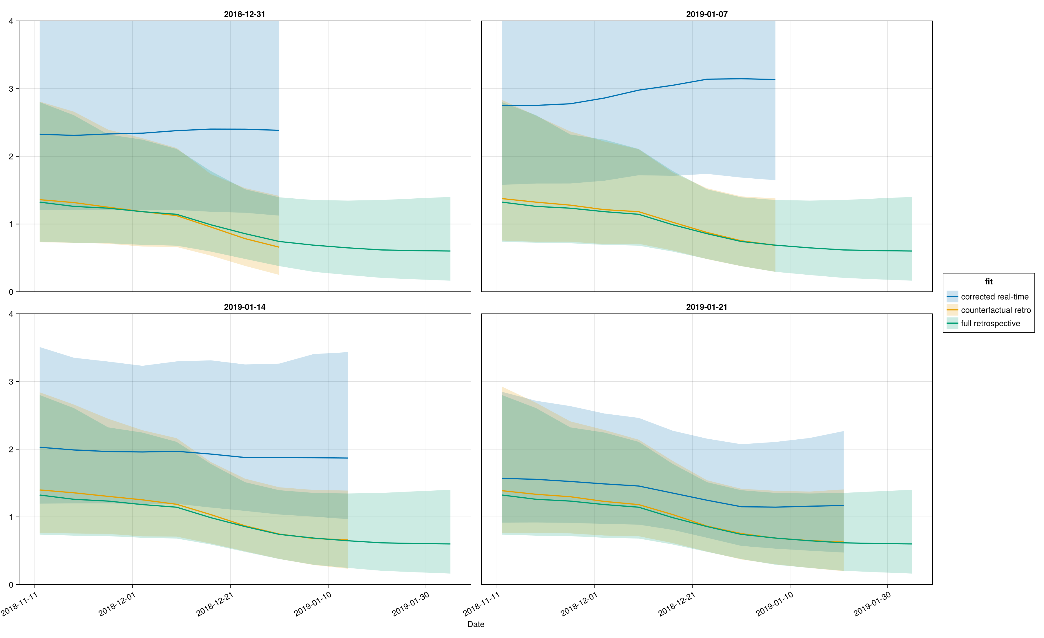
Population posteriors per cut-off
Overlaid marginals of (μ_inc, σ_inc, μ_δ, σ_δ, k) at each cut-off, one row per obs_date. If the corrected real-time density tracks the counterfactual retro density on each panel, the corrections are recovering the population from the truncated observations.
Long-form DataFrame of scalar parameter draws from a summarise posterior NamedTuple (one Vector{Float64} per param).
function post_long(post, params; obs_date, fit)
    rows = mapreduce(vcat, params) do p
        vals = getproperty(post, p)
        DataFrame(obs_date = string(obs_date), fit = fit,
            param = String(p), value = collect(vals))
    end
    return rows
end

joint_marginals_df = let
    params = [:μ_inc, :σ_inc, :μ_δ, :σ_δ, :k]
    df = @chain joint_fits begin
        map(_) do fit
            vcat(
                post_long(fit.post_truth, params;
                    obs_date = fit.obs_date,
                    fit = "counterfactual retro"),
                post_long(fit.post_rt, params;
                    obs_date = fit.obs_date,
                    fit = "corrected real-time"),
                post_long(post_retro_full, params;
                    obs_date = fit.obs_date,
                    fit = "full retrospective"))
        end
        reduce(vcat, _)
    end
    # Cap `k` at its 99% quantile (pooled across fits) so the long
    # right tail doesn't compress the other panels visually.
    k_cap = @chain df begin
        @rsubset :param == "k" && isfinite(:value)
        quantile(_.value, 0.99)
    end
    @rsubset(df, :param != "k" || :value <= k_cap)
end;

plot_marginal_overlay(joint_marginals_df;
    size_kw = (1800, 1300))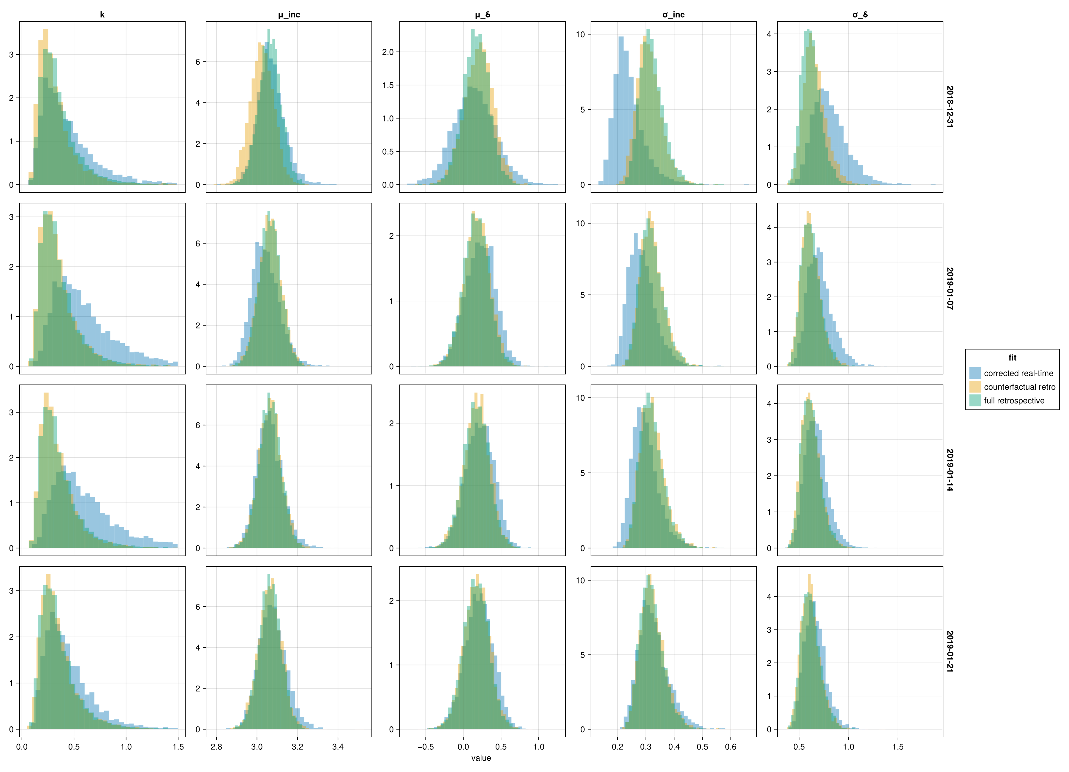
Controlled-outbreak projection
At each obs_date, three counterfactual predictions for the number of future symptomatic cases, each conditional on an assumed intervention rule. None of these scenarios is a factual claim about what happened in Epuyén; they describe what the fitted model implies if transmission had been interrupted in one of three ways.
Intervention on 2018-12-31 — transmission is assumed to have stopped on the onset date of the 18th case.
Intervention at the cut-off — transmission is assumed to have stopped at each panel's
obs_date. This ispredict_controlled_outbreak's default; for the Dec 31 panel it coincides with the variant above.No intervention — current sources keep transmitting; see
predict_natural_chain_outbreak.
The realised count of cases with onset strictly after each cut-off is overlaid as a vertical reference. It is one realisation drawn from the true (unknown) process; the predictive distribution is the posterior over what could have happened consistent with the fitted model and the assumed intervention rule, so we expect spread around the realised count rather than agreement on a point.
cutoff_18 = Date("2018-12-31")

function controlled_predictions(fit; corrected::Bool)
    strict = predict_controlled_outbreak(fit; corrected = corrected,
        obs_time = fit.obs_date,
        intervention_time = cutoff_18)
    at_obs = predict_controlled_outbreak(fit; corrected = corrected,
        obs_time = fit.obs_date)
    natural = predict_natural_chain_outbreak(fit;
        corrected = corrected,
        obs_time = fit.obs_date)
    (; fit.obs_date, fit.n_rt,
        strict_samples = strict.future_samples,
        at_obs_samples = at_obs.future_samples,
        natural_samples = natural.future_samples,
        at_obs_per_source = at_obs,
        actual_future = realised_future_count(ll, fit.obs_date))
end

controlled = [controlled_predictions(fit; corrected = true)
              for fit in joint_fits];
controlled_truth = [controlled_predictions(fit; corrected = false)
                    for fit in joint_fits];
Per-source breakdown for the intervention-at-cut-off counterfactual at the latest obs_date: shows which sources drive the projected future onset count, one row per observed source.
per_source_predictive_summary(controlled[end].at_obs_per_source)

function controlled_summary_df(pred)
    rows = map(pred) do c
        s = summarise_predictive(c.strict_samples)
        a = summarise_predictive(c.at_obs_samples)
        n = summarise_predictive(c.natural_samples)
        (obs_date = c.obs_date,
            n_obs = c.n_rt,
            actual_future = c.actual_future,
            strict_median = s.med,
            strict_lo10 = s.lo,
            strict_hi90 = s.hi,
            at_obs_median = a.med,
            at_obs_lo10 = a.lo,
            at_obs_hi90 = a.hi,
            natural_median = n.med,
            natural_lo10 = n.lo,
            natural_hi90 = n.hi)
    end
    DataFrame(rows)
end

controlled_df = controlled_summary_df(controlled)| Row | obs_date | n_obs | actual_future | strict_median | strict_lo10 | strict_hi90 | at_obs_median | at_obs_lo10 | at_obs_hi90 | natural_median | natural_lo10 | natural_hi90 |
|---|---|---|---|---|---|---|---|---|---|---|---|---|
| Date | Int64 | Int64 | Int64 | Int64 | Int64 | Int64 | Int64 | Int64 | Int64 | Int64 | Int64 | |
| 1 | 2018-12-31 | 18 | 16 | 22 | 9 | 51 | 22 | 9 | 51 | 25 | 10 | 59 |
| 2 | 2019-01-07 | 27 | 7 | 25 | 11 | 55 | 53 | 26 | 120 | 57 | 28 | 127 |
| 3 | 2019-01-14 | 29 | 5 | 6 | 2 | 13 | 25 | 11 | 50 | 26 | 13 | 52 |
| 4 | 2019-01-21 | 30 | 4 | 1 | 0 | 4 | 8 | 3 | 18 | 9 | 3 | 20 |
controlled_df_truth = controlled_summary_df(controlled_truth)| Row | obs_date | n_obs | actual_future | strict_median | strict_lo10 | strict_hi90 | at_obs_median | at_obs_lo10 | at_obs_hi90 | natural_median | natural_lo10 | natural_hi90 |
|---|---|---|---|---|---|---|---|---|---|---|---|---|
| Date | Int64 | Int64 | Int64 | Int64 | Int64 | Int64 | Int64 | Int64 | Int64 | Int64 | Int64 | |
| 1 | 2018-12-31 | 18 | 16 | 24 | 12 | 46 | 24 | 12 | 46 | 33 | 16 | 66 |
| 2 | 2019-01-07 | 27 | 7 | 12 | 5 | 24 | 27 | 13 | 56 | 34 | 16 | 72 |
| 3 | 2019-01-14 | 29 | 5 | 4 | 1 | 9 | 20 | 9 | 44 | 24 | 10 | 51 |
| 4 | 2019-01-21 | 30 | 4 | 1 | 0 | 3 | 9 | 4 | 19 | 12 | 5 | 25 |
The histogram below is drawn TWICE: once from the corrected real-time fit (what an analyst would see in real time) and once from the counterfactual retro fit (what a perfect-information analyst with exposure-aware filtering would see). Both use a 2×2 layout over obs_date to match the R(t) overlay panel above.
function plot_controlled_hist(pred; size_kw = (1500, 1200))
    kinds = [(:strict_samples, "intervention 2018-12-31"),
        (:at_obs_samples, "intervention at cut-off"),
        (:natural_samples, "no intervention")]
    df_hist = @chain pred begin
        mapreduce(vcat, _) do c
            mapreduce(vcat, kinds) do (field, label)
                DataFrame(panel = string(c.obs_date), kind = label,
                    value = Float64.(getproperty(c, field)))
            end
        end
        groupby(:panel)
        @transform :cap = quantile(:value, 0.99)
        @rsubset :value <= :cap
        @select :panel :kind :value
    end
    df_vline = @chain pred begin
        DataFrame(panel = string.(getfield.(_, :obs_date)),
            kind = "realised",
            value = Float64.(getfield.(_, :actual_future)))
    end
    hist_spec = data(df_hist) *
                mapping(:value => "Future cases";
                    color = :kind, layout = :panel) *
                visual(Hist; bins = 30, normalization = :pdf, alpha = 0.4)
    vline_spec = data(df_vline) *
                 mapping(:value; color = :kind, layout = :panel) *
                 visual(VLines; linewidth = 3)
    draw(hist_spec + vline_spec;
        facet = (linkxaxes = :none, linkyaxes = :none),
        figure = (; size = size_kw))
end
plot_controlled_hist (generic function with 1 method)Corrected real-time predictive distribution (top).
plot_controlled_hist(controlled)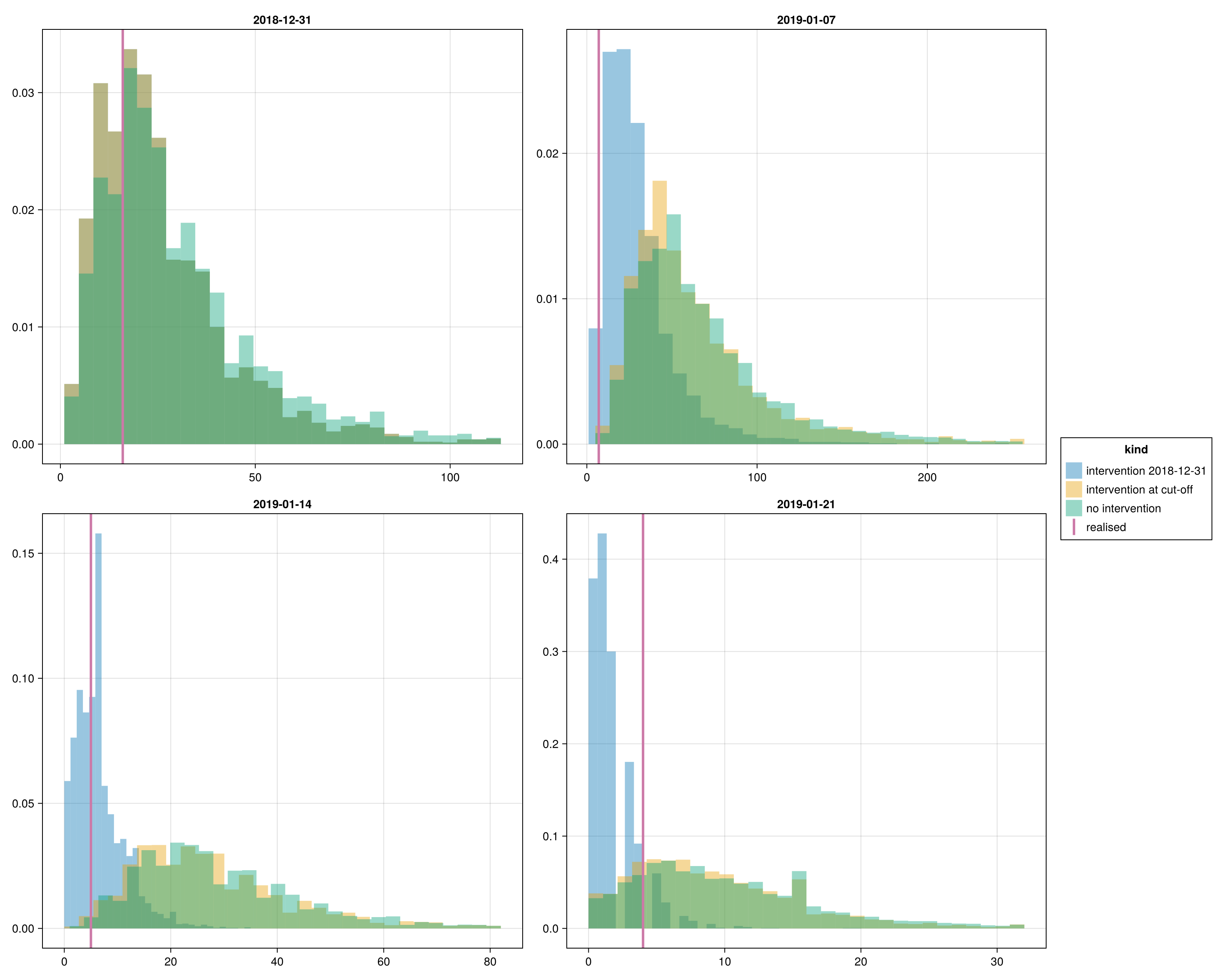
Counterfactual retro predictive distribution (below): same scenarios, but conditioned on the counterfactual retro fit at each cut-off.
plot_controlled_hist(controlled_truth)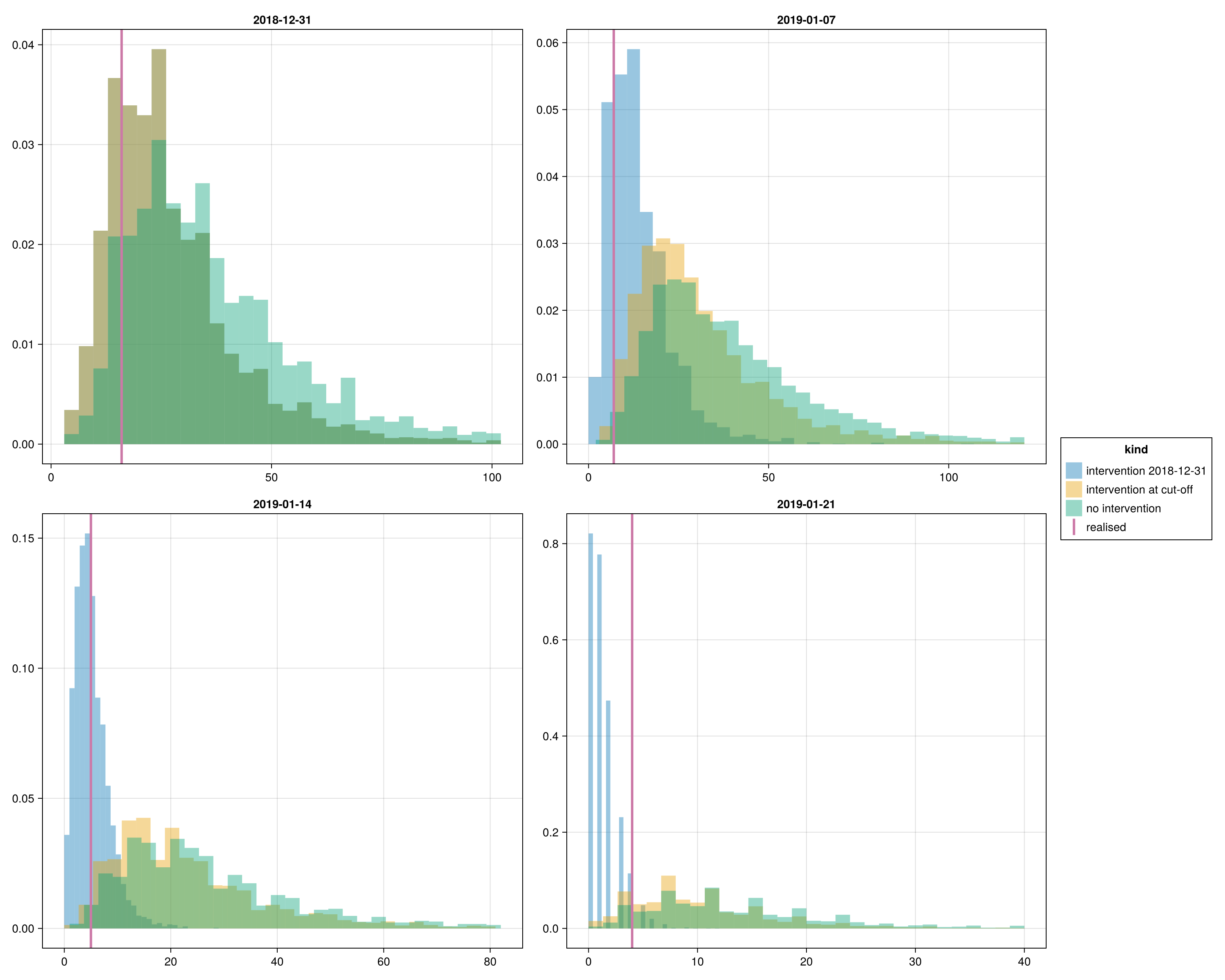
Why the Jan 7 predictive is wider than Dec 31, and how Jan 14 tightens
More data does not always mean a tighter future-cases prediction. At Jan 7 the line list adds secondary cases with onsets in the last week before the cut-off, so for those sources the chain is far from complete and most of their expected offspring still lies in the future. At Dec 31 the late-onset sources are fewer and most of their expected offspring chains have already completed, so each source contributes less to the future window. By Jan 14 the late-December sources have had two further weeks for their offspring to surface, so the completeness factor pins their per-source rate more tightly and the predictive distribution narrows even though the late-cut-off sources themselves remain pipeline-heavy. By Jan 21 the same is true of the early-January cohort, so the predictive tightens further toward the realised count.
Why the upper tail is wide even under the strict counterfactual
Under the assumed strict counterfactual we still expect a substantial pipeline from sources who became symptomatic just before the assumed intervention date. Their offspring chains were almost certainly initiated before the cut-off (the fitted transmission timing δ is centred near zero days post-source-onset), and most of those offspring would still be in the incubation period at obs_date. The wide upper band reflects two compounding sources of uncertainty: the R(t) posterior at the latest knots is wide because few cases inform it directly, and the small posterior of the dispersion k means even sources with no observed offspring carry meaningful pipeline mass. See the Limitations page for the real-time fitting caveats.
Per-source intervention rules
The scenarios above set a single intervention date (or none) that applies to every source. intervention_time also accepts a Vector{Date} of length N — one cut-off per observed source — for cases where isolation policies differ across individuals. An aggressive contact-tracing scenario in which each case is isolated on or shortly after their own symptom onset could be encoded by passing a per-source vector derived from ll_rt.onset_date. We do not have direct evidence of per-case isolation in the Epuyén outbreak so we do not run this scenario here, but the API supports it.