Simulation-based parameter recovery

Simulation-based recovery closes the loop between the joint model's generative side and its inference side: fix the population-level parameters to a known truth, simulate offspring counts Zobs from the resulting fixed model, then refit and check that the 95% posterior credible intervals cover the truth. This page runs one retrospective and one real-time variant at vignette scale; the unit-test suite extends the same pattern across more seeds and tighter budgets (see test/test_joint_recovery.jl).

Only log_R_init, σ_rw, and phi_inv_sqrt (equivalently k) are recoverable through this entry point. latent_times_model draws T_onset and T_inf from Uniform priors over per-case windows; the incubation and δ log-densities enter via @addlogprob!, which rand does not replay, so the simulated Z[i] ~ safe_nb(k, R_i) depends on the random-walk parameters and phi_inv_sqrt only. The delay parameters μ_inc, σ_inc, μ_δ, σ_δ are still fix-ed during simulation so the truth NamedTuple is coherent, and their recovery is exercised separately by test_recovery.jl and test_submodel_recovery.jl.

using TransmissionLinelist
using AlgebraOfGraphics: data, mapping, visual, draw
using DataFrames: DataFrame
using Dates: Date, Day
using Random: MersenneTwister
using Statistics: quantile
using CairoMakie
using CairoMakie: Hist, VLines
using Turing: DynamicPPL
using Logging: Logging

# Silence the NUTS "Found initial step size" Info logs.
Logging.disable_logging(Logging.Info)

LogLevel(1)

Truth

A single truth tuple drives both the retrospective and the real-time fit. Values match those in test/test_joint_recovery.jl so the vignette and the unit test exercise the same scenario. phi_inv_sqrt = 1/√4 corresponds to k = 4; σ_rw = 0.15 keeps the weekly random walk on log R(t) modest enough that the simulated outbreak does not blow up exponentially over the knot grid.

truth = (;
    μ_inc = 3.0, σ_inc = 0.45,
    μ_δ = 1.5, σ_δ = 1.2,
    log_R_init = log(1.4), σ_rw = 0.15,
    phi_inv_sqrt = 1.0 / sqrt(4.0))
truth_k = 1.0 / truth.phi_inv_sqrt^2
seed = 20260519

20260519

Sim → recover helper

Both variants follow the same three-step recipe: build a joint_model whose Zobs is missing so case_model samples Z[i] under the NB likelihood; fix the population parameters to truth; draw one set of simulated counts with rand; then refit the model on the simulated counts and return the chain.

function sim_and_refit(d_obs, edges; truth, seed)
    Zmiss = Vector{Union{Missing, Int}}(missing, d_obs.N)
    d_sim_in = merge(d_obs, (; Zobs = Zmiss))
    sim_model = joint_model(d_sim_in, edges)
    fixed = DynamicPPL.fix(sim_model, truth)
    sim = rand(MersenneTwister(seed), fixed)
    Z_sim = extract_simulated_Zobs(sim, d_obs.N)
    d_sim = merge(d_obs, (; Zobs = Z_sim))
    fit_model = joint_model(d_sim, edges)
    chn = sample_fit(fit_model; seed = seed)
    return (; chn, Z_sim)
end

sim_and_refit (generic function with 1 method)

Long-form DataFrame for one fit, with one row per (parameter, posterior draw). :k is reported on the natural scale so the truth overlay is on the same scale as the headline summaries elsewhere in the docs.

function posterior_long(chn; truth, truth_k)
    log_R_init = vec(collect(chn[:log_R_init]))
    σ_rw = vec(collect(chn[:σ_rw]))
    k = vec(collect(chn[:k]))
    truths = Dict("log_R_init" => truth.log_R_init,
        "σ_rw" => truth.σ_rw, "k" => truth_k)
    df = vcat(
        DataFrame(param = "log_R_init", value = log_R_init),
        DataFrame(param = "σ_rw", value = σ_rw),
        DataFrame(param = "k", value = k))
    df_truth = DataFrame(param = collect(keys(truths)),
        value = collect(values(truths)))
    return df, df_truth
end

posterior_long (generic function with 1 method)

Posterior histograms with a vertical reference line at the truth, one column per parameter. Lifted from plot_marginal_overlay's AoG pattern (data * mapping * visual(Hist)) with visual(VLines) for the truth overlay. Lives in the vignette for now; could be promoted to the package if a second page needs the same comparison.

function plot_posterior_vs_truth(df, df_truth; size_kw = (1500, 450))
    hist_spec = data(df) *
                mapping(:value => "value"; col = :param) *
                visual(Hist; bins = 30, normalization = :pdf,
                    color = (:steelblue, 0.55))
    vline_spec = data(df_truth) *
                 mapping(:value; col = :param) *
                 visual(VLines; color = :darkorange, linewidth = 3)
    draw(hist_spec + vline_spec;
        facet = (linkxaxes = :none, linkyaxes = :none),
        figure = (; size = size_kw))
end

plot_posterior_vs_truth (generic function with 1 method)

Coverage check for one fit: 95% CrI bounds for log_R_init, σ_rw, and k alongside the truth value and a covered flag.

function coverage_table(chn; truth, truth_k)
    rows = [
        ("log_R_init", vec(collect(chn[:log_R_init])), truth.log_R_init),
        ("σ_rw", vec(collect(chn[:σ_rw])), truth.σ_rw),
        ("k", vec(collect(chn[:k])), truth_k)
    ]
    DataFrame(map(rows) do (name, draws, truth_val)
        lo, hi = quantile(draws, [0.025, 0.975])
        (; param = name, truth = truth_val,
            lower_95 = lo, upper_95 = hi,
            covered = lo <= truth_val <= hi)
    end)
end

coverage_table (generic function with 1 method)

Retrospective sim → recover

d_obs reuses the bundled Epuyén line-list window structure (onset_lo_day, exp_lo_day, source_idx, …); only the observed offspring counts Zobs are re-simulated from the truth. With d.obs_time === nothing, truncation_model is a no-op, so the per-case rate reduces to R_i = exp(log_R_at(T_onset[i], edges, log_R)).

ll = load_linelist();
t0_ref = minimum(ll.onset_date) - Day(60)
d_retro = build_data(ll; t0 = t0_ref)
edges_retro = prepare_rt_edges(t0_ref)

retro = sim_and_refit(d_retro, edges_retro; truth, seed);

Retrospective coverage

coverage_table(retro.chn; truth, truth_k)

3×5 DataFrame

Row	param	truth	lower_95	upper_95	covered
	String	Float64	Float64	Float64	Bool
1	log_R_init	0.336472	-0.223569	0.991545	true
2	σ_rw	0.15	0.00627311	0.387906	true
3	k	4.0	2.72592	6138.26	true

Retrospective posterior vs truth

let (df, df_truth) = posterior_long(retro.chn; truth, truth_k)
    plot_posterior_vs_truth(df, df_truth)
end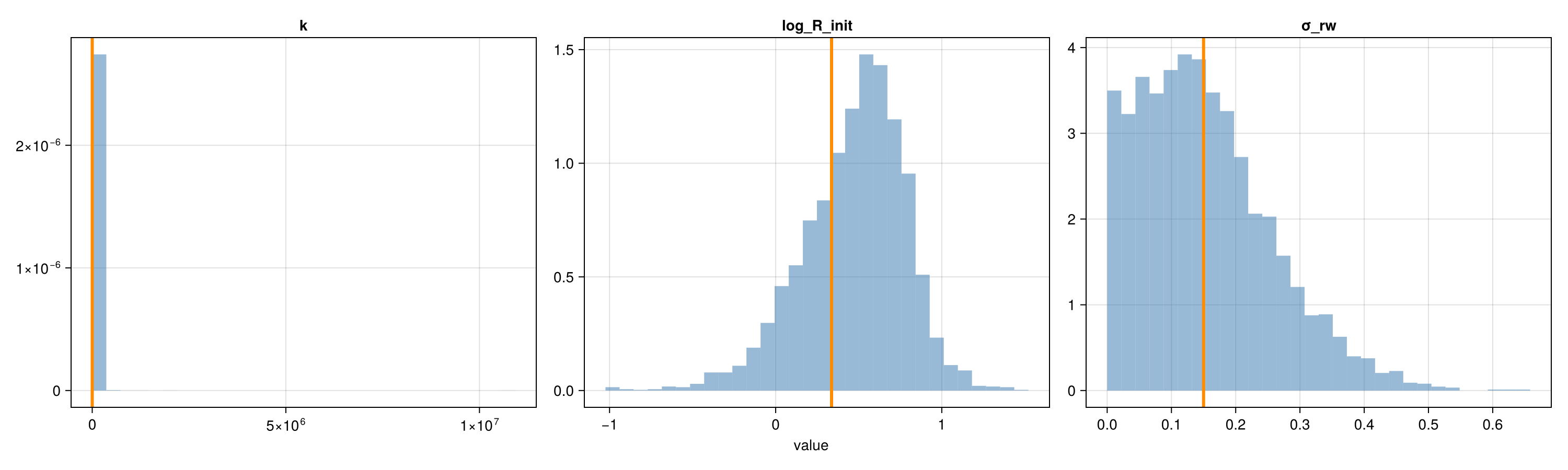

Real-time sim → recover

Same recipe at obs_date = Date("2018-12-31"). obs_time is set on the data tuple so truncation_model fires during both simulation and refit: incubation right-truncation for index cases, an offspring- completeness denominator for sourced cases, and the per-case R_eff = R_i · p_i thinning in case_model. Latent times are drawn from their Uniform priors during rand, so the truncation log-prob terms enter the simulation but do not change the sampled values of Z.

obs_date = Date("2018-12-31")
ll_rt = filter_realtime(ll, obs_date)
d_rt = build_data(ll_rt; obs_time = obs_date, t0 = t0_ref)
edges_rt = prepare_rt_edges(t0_ref; obs_time = obs_date)

realtime = sim_and_refit(d_rt, edges_rt; truth, seed);

Real-time coverage

coverage_table(realtime.chn; truth, truth_k)

3×5 DataFrame

Row	param	truth	lower_95	upper_95	covered
	String	Float64	Float64	Float64	Bool
1	log_R_init	0.336472	-0.486681	0.96664	true
2	σ_rw	0.15	0.00501812	0.419594	true
3	k	4.0	0.892417	4882.76	true

Real-time posterior vs truth

let (df, df_truth) = posterior_long(realtime.chn; truth, truth_k)
    plot_posterior_vs_truth(df, df_truth)
end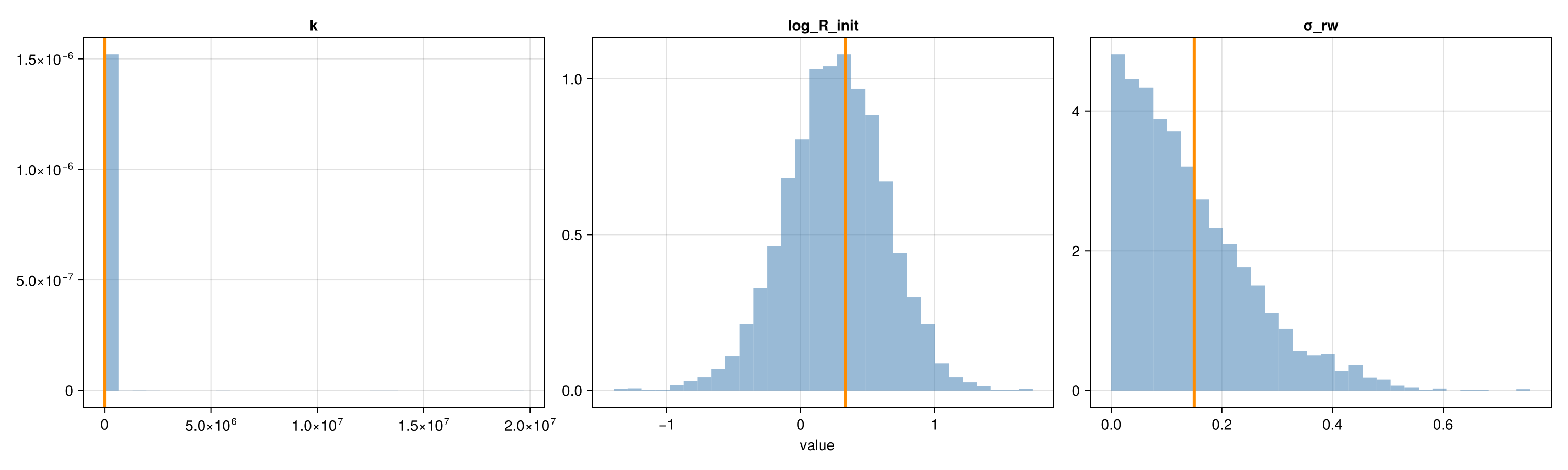

What to expect

Coverage of the 95% credible intervals on a single simulated dataset is itself stochastic — a single seed will miss the truth roughly once in twenty parameter-by-fit cells on average even when the model is correctly specified. A miss on a given run is informative: parameters where the prior dominates (here, σ_rw under the tight N⁺(0, 0.2) default and phi_inv_sqrt under N⁺(0, 1.0) with a small line list) can sit on the prior even when the truth is in the tail. For systematic coverage across seeds and budgets see test/test_joint_recovery.jl.