
Scoring multivariate forecasts
Source:vignettes/scoring-multivariate-forecasts.Rmd
scoring-multivariate-forecasts.RmdThis Vignette provides an overview about how to score multivariate forecasts.
Univariate forecasts
Let’s start with a simple univariate forecast: The number of cases of COVID-19 in Germany on 2021-05-15, forecasted by the EuroCOVIDhub-ensemble model on 2021-05-03. In our example, this forecast is represented by a set of 40 samples from the predictive distribution.
library(scoringutils)

example_univ_single <- example_sample_continuous[
  target_type == "Cases" &
    location == "DE" &
    forecast_date == "2021-05-03" &
    target_end_date == "2021-05-15" &
    horizon == 2 &
    model == "EuroCOVIDhub-ensemble"
]
example_univ_single
#> Forecast type: sample
#> Forecast unit:
#> location, location_name, target_end_date, target_type, forecast_date, model,
#> and horizon
#>
#>     location location_name target_end_date target_type forecast_date
#>       <char>        <char>          <Date>      <char>        <Date>
#>  1:       DE       Germany      2021-05-15       Cases    2021-05-03
#>  2:       DE       Germany      2021-05-15       Cases    2021-05-03
#>  3:       DE       Germany      2021-05-15       Cases    2021-05-03
#>  4:       DE       Germany      2021-05-15       Cases    2021-05-03
#>  5:       DE       Germany      2021-05-15       Cases    2021-05-03
#>  6:       DE       Germany      2021-05-15       Cases    2021-05-03
#>  7:       DE       Germany      2021-05-15       Cases    2021-05-03
#>  8:       DE       Germany      2021-05-15       Cases    2021-05-03
#>  9:       DE       Germany      2021-05-15       Cases    2021-05-03
#> 10:       DE       Germany      2021-05-15       Cases    2021-05-03
#> 11:       DE       Germany      2021-05-15       Cases    2021-05-03
#> 12:       DE       Germany      2021-05-15       Cases    2021-05-03
#> 13:       DE       Germany      2021-05-15       Cases    2021-05-03
#> 14:       DE       Germany      2021-05-15       Cases    2021-05-03
#> 15:       DE       Germany      2021-05-15       Cases    2021-05-03
#> 16:       DE       Germany      2021-05-15       Cases    2021-05-03
#> 17:       DE       Germany      2021-05-15       Cases    2021-05-03
#> 18:       DE       Germany      2021-05-15       Cases    2021-05-03
#> 19:       DE       Germany      2021-05-15       Cases    2021-05-03
#> 20:       DE       Germany      2021-05-15       Cases    2021-05-03
#> 21:       DE       Germany      2021-05-15       Cases    2021-05-03
#> 22:       DE       Germany      2021-05-15       Cases    2021-05-03
#> 23:       DE       Germany      2021-05-15       Cases    2021-05-03
#> 24:       DE       Germany      2021-05-15       Cases    2021-05-03
#> 25:       DE       Germany      2021-05-15       Cases    2021-05-03
#> 26:       DE       Germany      2021-05-15       Cases    2021-05-03
#> 27:       DE       Germany      2021-05-15       Cases    2021-05-03
#> 28:       DE       Germany      2021-05-15       Cases    2021-05-03
#> 29:       DE       Germany      2021-05-15       Cases    2021-05-03
#> 30:       DE       Germany      2021-05-15       Cases    2021-05-03
#> 31:       DE       Germany      2021-05-15       Cases    2021-05-03
#> 32:       DE       Germany      2021-05-15       Cases    2021-05-03
#> 33:       DE       Germany      2021-05-15       Cases    2021-05-03
#> 34:       DE       Germany      2021-05-15       Cases    2021-05-03
#> 35:       DE       Germany      2021-05-15       Cases    2021-05-03
#> 36:       DE       Germany      2021-05-15       Cases    2021-05-03
#> 37:       DE       Germany      2021-05-15       Cases    2021-05-03
#> 38:       DE       Germany      2021-05-15       Cases    2021-05-03
#> 39:       DE       Germany      2021-05-15       Cases    2021-05-03
#> 40:       DE       Germany      2021-05-15       Cases    2021-05-03
#>     location location_name target_end_date target_type forecast_date
#>       <char>        <char>          <Date>      <char>        <Date>
#>                     model horizon predicted sample_id observed
#>                    <char>   <num>     <num>     <int>    <num>
#>  1: EuroCOVIDhub-ensemble       2 109365.73         1    64985
#>  2: EuroCOVIDhub-ensemble       2  63041.27         2    64985
#>  3: EuroCOVIDhub-ensemble       2 186364.05         3    64985
#>  4: EuroCOVIDhub-ensemble       2 127841.64         4    64985
#>  5: EuroCOVIDhub-ensemble       2  79550.56         5    64985
#>  6: EuroCOVIDhub-ensemble       2 193981.34         6    64985
#>  7: EuroCOVIDhub-ensemble       2 122953.97         7    64985
#>  8: EuroCOVIDhub-ensemble       2 148088.41         8    64985
#>  9: EuroCOVIDhub-ensemble       2 104570.23         9    64985
#> 10: EuroCOVIDhub-ensemble       2 130718.45        10    64985
#> 11: EuroCOVIDhub-ensemble       2 154126.24        11    64985
#> 12: EuroCOVIDhub-ensemble       2 164671.65        12    64985
#> 13: EuroCOVIDhub-ensemble       2 118330.18        13    64985
#> 14: EuroCOVIDhub-ensemble       2 107950.08        14    64985
#> 15: EuroCOVIDhub-ensemble       2 151033.84        15    64985
#> 16: EuroCOVIDhub-ensemble       2 120649.63        16    64985
#> 17: EuroCOVIDhub-ensemble       2 114380.55        17    64985
#> 18: EuroCOVIDhub-ensemble       2 104300.98        18    64985
#> 19: EuroCOVIDhub-ensemble       2 144538.28        19    64985
#> 20: EuroCOVIDhub-ensemble       2  66689.95        20    64985
#> 21: EuroCOVIDhub-ensemble       2 131096.85        21    64985
#> 22: EuroCOVIDhub-ensemble       2 120698.00        22    64985
#> 23: EuroCOVIDhub-ensemble       2 199890.08        23    64985
#> 24: EuroCOVIDhub-ensemble       2 132037.17        24    64985
#> 25: EuroCOVIDhub-ensemble       2  89928.75        25    64985
#> 26: EuroCOVIDhub-ensemble       2 144859.42        26    64985
#> 27: EuroCOVIDhub-ensemble       2 148745.59        27    64985
#> 28: EuroCOVIDhub-ensemble       2  97248.30        28    64985
#> 29: EuroCOVIDhub-ensemble       2  73744.04        29    64985
#> 30: EuroCOVIDhub-ensemble       2 117133.25        30    64985
#> 31: EuroCOVIDhub-ensemble       2 197014.73        31    64985
#> 32: EuroCOVIDhub-ensemble       2 137847.82        32    64985
#> 33: EuroCOVIDhub-ensemble       2 120085.18        33    64985
#> 34: EuroCOVIDhub-ensemble       2  91030.07        34    64985
#> 35: EuroCOVIDhub-ensemble       2 133265.23        35    64985
#> 36: EuroCOVIDhub-ensemble       2 161345.08        36    64985
#> 37: EuroCOVIDhub-ensemble       2  52633.20        37    64985
#> 38: EuroCOVIDhub-ensemble       2 104926.13        38    64985
#> 39: EuroCOVIDhub-ensemble       2 162582.41        39    64985
#> 40: EuroCOVIDhub-ensemble       2 143421.88        40    64985
#>                     model horizon predicted sample_id observed
#>                    <char>   <num>     <num>     <int>    <num>
We can score this forecast and will receive a single score.
score(example_univ_single)
#>    location location_name target_end_date target_type forecast_date
#>      <char>        <char>          <Date>      <char>        <Date>
#> 1:       DE       Germany      2021-05-15       Cases    2021-05-03
#>                    model horizon  bias      dss     crps overprediction
#>                   <char>   <num> <num>    <num>    <num>          <num>
#> 1: EuroCOVIDhub-ensemble       2   0.9 24.00559 42655.41       34690.28
#>    underprediction dispersion log_score      mad ae_median    se_mean
#>              <num>      <num>     <num>    <num>     <num>      <num>
#> 1:               0   7965.135  12.64899 31078.55   60412.8 3823196821
Now, of course, we can also score multiple similar forecasts at the same time. Let’s say we’re not only interested in Germany, but other countries as well.
example_univ_multi <- example_sample_continuous[
  target_type == "Cases" &
    forecast_date == "2021-05-03" &
    target_end_date == "2021-05-15" &
    horizon == 2 &
    model == "EuroCOVIDhub-ensemble"
]
example_univ_multi
#> Forecast type: sample
#> Forecast unit:
#> location, location_name, target_end_date, target_type, forecast_date, model,
#> and horizon
#>
#>      location location_name target_end_date target_type forecast_date
#>        <char>        <char>          <Date>      <char>        <Date>
#>   1:       DE       Germany      2021-05-15       Cases    2021-05-03
#>   2:       DE       Germany      2021-05-15       Cases    2021-05-03
#>   3:       DE       Germany      2021-05-15       Cases    2021-05-03
#>   4:       DE       Germany      2021-05-15       Cases    2021-05-03
#>   5:       DE       Germany      2021-05-15       Cases    2021-05-03
#>  ---
#> 156:       IT         Italy      2021-05-15       Cases    2021-05-03
#> 157:       IT         Italy      2021-05-15       Cases    2021-05-03
#> 158:       IT         Italy      2021-05-15       Cases    2021-05-03
#> 159:       IT         Italy      2021-05-15       Cases    2021-05-03
#> 160:       IT         Italy      2021-05-15       Cases    2021-05-03
#>                      model horizon predicted sample_id observed
#>                     <char>   <num>     <num>     <int>    <num>
#>   1: EuroCOVIDhub-ensemble       2 109365.73         1    64985
#>   2: EuroCOVIDhub-ensemble       2  63041.27         2    64985
#>   3: EuroCOVIDhub-ensemble       2 186364.05         3    64985
#>   4: EuroCOVIDhub-ensemble       2 127841.64         4    64985
#>   5: EuroCOVIDhub-ensemble       2  79550.56         5    64985
#>  ---
#> 156: EuroCOVIDhub-ensemble       2  72194.00        36    50453
#> 157: EuroCOVIDhub-ensemble       2  82507.14        37    50453
#> 158: EuroCOVIDhub-ensemble       2 102956.27        38    50453
#> 159: EuroCOVIDhub-ensemble       2  55985.84        39    50453
#> 160: EuroCOVIDhub-ensemble       2  65929.64        40    50453
Now, we have a set of 4 forecasts for 4 different countries, each of them represented by a set of 40 samples from the predictive distribution.
When we score these forecasts, we will get 4 scores, one for each forecast and observed value.
score(example_univ_multi)
#>    location  location_name target_end_date target_type forecast_date
#>      <char>         <char>          <Date>      <char>        <Date>
#> 1:       DE        Germany      2021-05-15       Cases    2021-05-03
#> 2:       FR         France      2021-05-15       Cases    2021-05-03
#> 3:       GB United Kingdom      2021-05-15       Cases    2021-05-03
#> 4:       IT          Italy      2021-05-15       Cases    2021-05-03
#>                    model horizon  bias      dss      crps overprediction
#>                   <char>   <num> <num>    <num>     <num>          <num>
#> 1: EuroCOVIDhub-ensemble       2  0.90 24.00559 42655.413       34690.28
#> 2: EuroCOVIDhub-ensemble       2  0.50 22.37188 21960.030        7820.70
#> 3: EuroCOVIDhub-ensemble       2 -0.60 17.19740  2334.652           0.00
#> 4: EuroCOVIDhub-ensemble       2  0.95 21.73164 16262.604       12531.20
#>    underprediction dispersion log_score       mad ae_median    se_mean
#>              <num>      <num>     <num>     <num>     <num>      <num>
#> 1:           0.000  7965.1347  12.64899 31078.550 60412.802 3823196821
#> 2:           0.000 14139.3296  11.99198 57243.099 38228.018 1763097632
#> 3:        1629.644   705.0089  10.03031  2680.797  3902.441   10157513
#> 4:           0.000  3731.3990  11.57288 16954.657 23892.603  626560551
Multivariate forecasts
Now, instead of treating the four observations as independent, we could also think of them as a single realisation of a draw from the multivariate distribution of COVID-19 cases across several countries.
The corresponding multivariate forecast would similarly specify a predictive distribution for the number of cases across all 4 countries. The samples are then not draws from four independent distributions, but instead samples from a joint multivariate predictive distribution.
In the following, let’s assume that our samples were draws from a multivariate distribution all along (we just treated them as independent for the univariate case).
Note on the demonstration. The forecasts used in this vignette are for demonstration only and do not represent joint draws of a multivariate distribution. This means the dependence structure scored by multivariate scoring is more an artefact of how the data were prepared than a property of the original forecasts. (See
create-example-data.Rin theinst/folder for detail.)
To tell scoringutils that we want to treat these as a
multivariate forecast, we need to specify the columns that are pooled
together to form a single multivariate forecast. We do this via the
joint_across argument. For example, if we want to pool
forecasts across locations and treat them as a single multivariate
forecast, we could set
joint_across = c("location", "location_name") (in our
example, the two columns contain essentially the same information - we
therefore have to include both in joint_across (or could
alternatively delete one of them)).
example_multiv <- as_forecast_multivariate_sample(
  data = example_univ_multi,
  c("location", "location_name")
)
example_multiv
#> Forecast type: multivariate_sample
#> Forecast unit:
#> location, location_name, target_end_date, target_type, forecast_date, model,
#> and horizon
#> Joint across:
#> location and location_name
#>
#>      location location_name target_end_date target_type forecast_date
#>        <char>        <char>          <Date>      <char>        <Date>
#>   1:       DE       Germany      2021-05-15       Cases    2021-05-03
#>   2:       DE       Germany      2021-05-15       Cases    2021-05-03
#>   3:       DE       Germany      2021-05-15       Cases    2021-05-03
#>   4:       DE       Germany      2021-05-15       Cases    2021-05-03
#>   5:       DE       Germany      2021-05-15       Cases    2021-05-03
#>  ---
#> 156:       IT         Italy      2021-05-15       Cases    2021-05-03
#> 157:       IT         Italy      2021-05-15       Cases    2021-05-03
#> 158:       IT         Italy      2021-05-15       Cases    2021-05-03
#> 159:       IT         Italy      2021-05-15       Cases    2021-05-03
#> 160:       IT         Italy      2021-05-15       Cases    2021-05-03
#>                      model horizon predicted sample_id observed .mv_group_id
#>                     <char>   <num>     <num>     <int>    <num>        <int>
#>   1: EuroCOVIDhub-ensemble       2 109365.73         1    64985            1
#>   2: EuroCOVIDhub-ensemble       2  63041.27         2    64985            1
#>   3: EuroCOVIDhub-ensemble       2 186364.05         3    64985            1
#>   4: EuroCOVIDhub-ensemble       2 127841.64         4    64985            1
#>   5: EuroCOVIDhub-ensemble       2  79550.56         5    64985            1
#>  ---
#> 156: EuroCOVIDhub-ensemble       2  72194.00        36    50453            1
#> 157: EuroCOVIDhub-ensemble       2  82507.14        37    50453            1
#> 158: EuroCOVIDhub-ensemble       2 102956.27        38    50453            1
#> 159: EuroCOVIDhub-ensemble       2  55985.84        39    50453            1
#> 160: EuroCOVIDhub-ensemble       2  65929.64        40    50453            1
The column .mv_group_id is created automatically and
represents an identifier for each multivariate forecast.
.mv_group_id is 1 everywhere, because we only have a single
multivariate forecast. When scoring this forecast using an appropriate
multivariate scoring function, we will get a single score, even though
we have 4 observations, one for each country. (Note that for the
purposes of scoring, it doesn’t matter that sample ids are still 1-40,
repeated 4 times, instead of 1-160. scoringutils handles
this appropriately.)
score(example_multiv)
#>    target_end_date target_type forecast_date                 model horizon
#>             <Date>      <char>        <Date>                <char>   <num>
#> 1:      2021-05-15       Cases    2021-05-03 EuroCOVIDhub-ensemble       2
#>    energy_score variogram_score .mv_group_id
#>           <num>           <num>        <int>
#> 1:     54795.73        68523.93            1
By default, score() computes both the energy score and
the variogram score for multivariate sample forecasts. The energy score
is a multivariate generalisation of the CRPS that measures overall
forecast accuracy. The variogram score (Scheuerer and Hamill, 2015)
specifically targets the correlation structure between the targets being
forecast jointly. For each pair of targets (e.g. two countries), it
compares the observed absolute difference |y_i - y_j|^p against what the
forecast distribution predicts for that difference. A forecast that gets
the correlations between targets wrong will predict pairwise differences
that do not match the observations, producing a higher score. This makes
the variogram score more sensitive to misspecified correlations than the
energy score.
You can customise parameters using purrr::partial(). The
order parameter p controls how differences are scaled:
p = 0.5 (the default) is more robust to outliers, while
p = 1 gives a standard absolute difference. See
?variogram_score_multivariate for full parameter
documentation. For example, to use p = 1:
score(
  example_multiv,
  metrics = list(
    energy_score = energy_score_multivariate,
    variogram_score = purrr::partial( # nolint: namespace_linter.
      variogram_score_multivariate, p = 1
    )
  )
)
#>    target_end_date target_type forecast_date                 model horizon
#>             <Date>      <char>        <Date>                <char>   <num>
#> 1:      2021-05-15       Cases    2021-05-03 EuroCOVIDhub-ensemble       2
#>    energy_score variogram_score .mv_group_id
#>           <num>           <num>        <int>
#> 1:     54795.73     20111809605            1
A set of multivariate targets can be pooled to account for different
correlation structures. If, at any point, you want to score the same
forecast using different groupings, you’d have create a new separate
forecast object with a different grouping and score that new forecast
object. For example, to pool across horizons, we bring
target_end_date along with horizon, because
the two both vary within a trajectory.
example_cases <- na.omit(
  example_sample_continuous[
    target_type == "Cases" &
      model == "EuroCOVIDhub-ensemble"
  ]
)

example_traj <- as_forecast_multivariate_sample(
  data = example_cases,
  joint_across = c("horizon", "target_end_date")
)

head(score(example_traj), 3)
#>    location location_name target_type forecast_date                 model
#>      <char>        <char>      <char>        <Date>                <char>
#> 1:       DE       Germany       Cases    2021-05-03 EuroCOVIDhub-ensemble
#> 2:       DE       Germany       Cases    2021-05-10 EuroCOVIDhub-ensemble
#> 3:       DE       Germany       Cases    2021-05-17 EuroCOVIDhub-ensemble
#>    energy_score variogram_score .mv_group_id
#>           <num>           <num>        <int>
#> 1:     62512.17       40013.423            1
#> 2:     45118.99        6119.925            2
#> 3:     16761.77       12371.387            3
Each single score now covers one whole trajectory over three horizons.
Multivariate point forecasts
If you have point forecasts rather than samples, you can score them
using the variogram score via
as_forecast_multivariate_point(). This treats each point
forecast as a single-sample ensemble.
example_point_multi <- example_point[
  target_type == "Cases" &
    forecast_date == "2021-05-03" &
    target_end_date == "2021-05-15" &
    horizon == 2 &
    model == "EuroCOVIDhub-ensemble"
]

example_mv_point <- as_forecast_multivariate_point(
  data = na.omit(example_point_multi),
  joint_across = c("location", "location_name")
)
score(example_mv_point)
#>    target_end_date target_type forecast_date                 model horizon
#>             <Date>      <char>        <Date>                <char>   <num>
#> 1:      2021-05-15       Cases    2021-05-03 EuroCOVIDhub-ensemble       2
#>    variogram_score .mv_group_id
#>              <num>        <int>
#> 1:        51406.03            1
Multivariate quantile forecasts
Both the energy score and the variogram score need samples drawn from
the joint predictive distribution. We cannot use the same multivariate
scoring for quantile forecasts as they do not describe the relationship
between targets in this way. It is tempting to line the quantile levels
up across targets and treat them as samples (for instance by passing
sample_id = "quantile_level" to
as_forecast_multivariate_sample()).
scoringutils will warn you about the leftover
quantile_level column, but it will still return a score.
However that score is not the one you want, as in this case, every
quantile forecast ends up scored as though it had predicted perfect
dependence (regardless of what the underlying model actually
predicted).
Comparing the energy and variogram scores
The energy and variogram scores are complementary to each other. The
energy score summarises overall accuracy across all the pooled targets
at once, a multivariate generalisation of the CRPS. The variogram score
instead looks only at the differences between the specific targets that
were pooled together to compare the size of the observed difference
against the size of predicted differences. It is pairwise on whatever
dimension joint_across specified.
For example, when pooling across forecast horizon, the variogram compares the differences between weeks and is therefore sensitive to the shape of the trajectory. But because it uses only differences between targets, it is insensitive to any bias that shifts the overall trajectory away from the observed data.
We can see this comparison between the two scores, comparing two models’ forecasts of 1-3 week ahead cases in Germany as above. The dashed line shows the observed trajectory, with cases falling after the first week.
library(ggplot2)
library(data.table)
#>
#> Attaching package: 'data.table'
#> The following object is masked from 'package:base':
#>
#>     %notin%

cases_de <- as.data.table(example_sample_continuous)[
  target_type == "Cases" &
    location == "DE" &
    forecast_date == "2021-05-03" &
    model %in% c("EuroCOVIDhub-ensemble", "epiforecasts-EpiNow2")
]

band <- cases_de[, .(
  median = median(predicted),
  lower = quantile(predicted, 0.25),
  upper = quantile(predicted, 0.75)
), by = .(model, target_end_date)]

observed <- unique(cases_de[, .(target_end_date, observed)])

ggplot(band, aes(target_end_date, median, colour = model, fill = model)) +
  geom_ribbon(aes(ymin = lower, ymax = upper), alpha = 0.2, colour = NA) +
  geom_line() +
  geom_line(
    data = observed, aes(target_end_date, observed),
    inherit.aes = FALSE, linetype = "dashed"
  ) +
  geom_point(
    data = observed, aes(target_end_date, observed),
    inherit.aes = FALSE
  ) +
  labs(x = "Target date", y = "Weekly cases", colour = "Model", fill = "Model") +
  theme_scoringutils() +
  theme(legend.position = "bottom")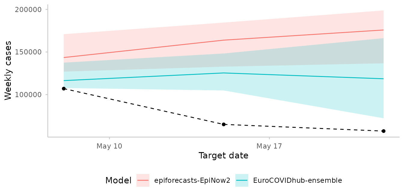
We pool the three horizons into a single multivariate forecast for each model, then score both.
cases_mv <- as_forecast_multivariate_sample(
  data = na.omit(cases_de),
  joint_across = c("horizon", "target_end_date")
)
score(cases_mv)[, c("model", "energy_score", "variogram_score")]
#>                    model energy_score variogram_score
#>                   <char>        <num>           <num>
#> 1: EuroCOVIDhub-ensemble     62512.17        40013.42
#> 2:  epiforecasts-EpiNow2    123346.17        30397.39
The two scores disagree about which model performed better. The energy score prefers the ensemble, whose level stays close to the observed cases, while the variogram score prefers EpiNow2. The observed cases move sharply from week to week, and EpiNow2 predicts changes of a similar size, whereas the near-flat ensemble predicts changes that are too small. Note that EpiNow2 wins on the variogram score even though it has the wrong direction of the change. The energy score rewards getting the overall level right; the variogram score rewards getting the size of the joint movement right.