Determines bias of quantile forecasts — bias

Determines bias from quantile forecasts. For an increasing number of quantiles this measure converges against the sample based bias version for integer and continuous forecasts.

Usage

bias_quantile(observed, predicted, quantile_level, na.rm = TRUE)

Arguments

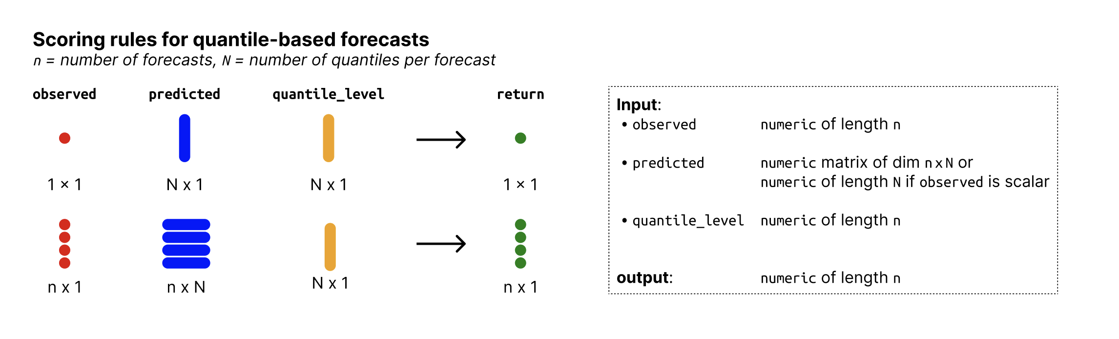
observed: Numeric vector of size n with the observed values.
predicted: Numeric nxN matrix of predictive quantiles, n (number of rows) being the number of forecasts (corresponding to the number of observed values) and N (number of columns) the number of quantiles per forecast. If observed is just a single number, then predicted can just be a vector of size N.
quantile_level: Vector of of size N with the quantile levels for which predictions were made. Note that if this does not contain the median (0.5) then the median is imputed as being the mean of the two innermost quantiles.
na.rm: Logical. Should missing values be removed?

Value

scalar with the quantile bias for a single quantile prediction

Details

For quantile forecasts, bias is measured as

$$ B_t = (1 - 2 \cdot \max \{i | q_{t,i} \in Q_t \land q_{t,i} \leq x_t\}) \mathbf{1}( x_t \leq q_{t, 0.5}) \\ + (1 - 2 \cdot \min \{i | q_{t,i} \in Q_t \land q_{t,i} \geq x_t\}) 1( x_t \geq q_{t, 0.5}),$$

where $Q_t$ is the set of quantiles that form the predictive distribution at time $t$ and $x_t$ is the observed value. For consistency, we define $Q_t$ such that it always includes the element $q_{t, 0} = - \infty$ and $q_{t,1} = \infty$. $1()$ is the indicator function that is $1$ if the condition is satisfied and $0$ otherwise.

In clearer terms, bias $B_t$ is:

$1 - 2 \cdot$ the maximum percentile rank for which the corresponding quantile is still smaller than or equal to the observed value, if the observed value is smaller than the median of the predictive distribution.
$1 - 2 \cdot$ the minimum percentile rank for which the corresponding quantile is still larger than or equal to the observed value if the observed value is larger than the median of the predictive distribution..
$0$ if the observed value is exactly the median (both terms cancel out)

Bias can assume values between -1 and 1 and is 0 ideally (i.e. unbiased).

Note that if the given quantiles do not contain the median, the median is imputed as a linear interpolation of the two innermost quantiles. If the median is not available and cannot be imputed, an error will be thrown. Note that in order to compute bias, quantiles must be non-decreasing with increasing quantile levels.

For a large enough number of quantiles, the percentile rank will equal the proportion of predictive samples below the observed value, and the bias metric coincides with the one for continuous forecasts (see bias_sample()).

Input format

Examples

predicted <- matrix(c(1.5:23.5, 3.3:25.3), nrow = 2, byrow = TRUE)
quantile_level <- c(0.01, 0.025, seq(0.05, 0.95, 0.05), 0.975, 0.99)
observed <- c(15, 12.4)
bias_quantile(observed, predicted, quantile_level)
#> [1] -0.3  0.2