Sensitivity: model by horizon specification

Code
library(here)
library(dplyr)
library(tidyr)
library(purrr)
library(ggplot2)
library(knitr)
source(here("R", "sensitivity", "check-horizon-spec.R"))
specs <- read_horizon_specs()
arm_labels <- c(
  "additive" = "No interaction",
  "by-model" = "Separate curves (current)",
  "sz" = "Sum-to-zero deviations",
  "sz + model re" = "Sum-to-zero deviations + model level",
  "fs" = "Penalised deviations",
  "fs k4" = "Penalised deviations, k = 4",
  "factor re" = "Horizon as categories"
)
current <- arm_labels[["by-model"]]

Rationale

Code
coverage <- load_horizon_data() |>
  group_by(Model) |>
  summarise(n_horizons = n_distinct(Horizon), max_horizon = max(Horizon),
            forecasts = n())
partial <- filter(coverage, n_horizons < 4)

One of the most unsettled parts of our model specification was how we accounted for variation between individual models, and/or/with the length of forecast horizon. We have 48 individual models, predicting for any of {1, 2, 3, 4} weeks’ horizon.

This is also complicated by finding (rather late) that 8 of 48 models did not forecast all four horizons. We originally specified that these would be excluded, but it turns out I hadn’t implemented that properly so these have accidentally always been in our analysis (#180). Assuming we now want to keep these in, it makes checking the specification of model/horizon question slightly more relevant.

Assumptions

We have a strong prior belief that forecast performance degrades with increasing horizon.

Each treatment of horizon encodes a prior belief about the shape of the shared curve, from none (factor) to no horizon effect at all (flat).

Code
h <- 1:4
hf <- seq(1, 4, length.out = 100)
shape_labels <- c(
  "Factor\nno belief about shape",
  "Smooth, k = 4\nany shape, preferring a straight line",
  "Smooth, k = 3\nstraight line plus at most one bend",
  "Linear\nequal steps between horizons",
  "Flat\nhorizon has no effect",
  "Monotone ordinal\nerror never falls with horizon"
)
shape_fns <- list(
  NULL,
  \(x) 0.9 * plogis(4 * (x - 2.5)),
  \(x) 0.88 * log(x) / log(4),
  \(x) 0.3 * (x - 1),
  \(x) rep(0.45, length(x))
)
shape_lines <- map2_dfr(shape_fns[2:5], shape_labels[2:5],
                        \(f, p) tibble(p = p, x = hf, y = f(hf)))
shape_points <- bind_rows(
  tibble(p = shape_labels[1], x = h, y = c(0.1, 0.5, 0.35, 0.9)),
  map2_dfr(shape_fns[2:5], shape_labels[2:5], \(f, p) tibble(p = p, x = h, y = f(h))),
  tibble(p = shape_labels[6], x = h, y = c(0.05, 0.2, 0.85, 0.9))
)
shape_steps <- tibble(p = shape_labels[6], x = c(1, 2, 3, 4, 4.3),
                      y = c(0.05, 0.2, 0.85, 0.9, 0.9))
ggplot(mapping = aes(x, y)) +
  geom_path(data = shape_lines, colour = "firebrick", linewidth = 1) +
  geom_step(data = shape_steps, colour = "firebrick", linewidth = 1) +
  geom_point(data = shape_points, size = 2) +
  facet_wrap(~ factor(p, shape_labels), ncol = 3) +
  scale_x_continuous(breaks = 1:4, limits = c(0.8, 4.3)) +
  scale_y_continuous(limits = c(0, 1)) +
  labs(x = "Horizon (weeks)", y = "Log LWIS (schematic)") +
  theme_minimal() +
  theme(axis.text.y = element_blank(), panel.grid.minor = element_blank(),
        strip.text = element_text(hjust = 0))
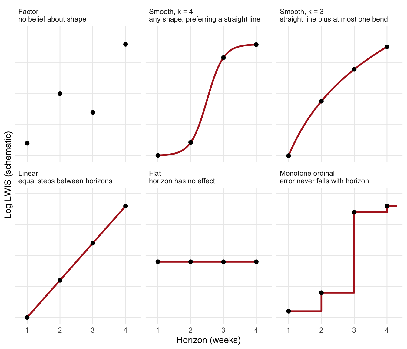
Prior belief about the shared horizon curve encoded by each treatment of horizon, weakest to strongest. Monotone is a different kind of constraint, not on this scale. Schematic, not fitted.

An ordered factor in R changes only the contrasts, not the fit, so it does not use the ordering.

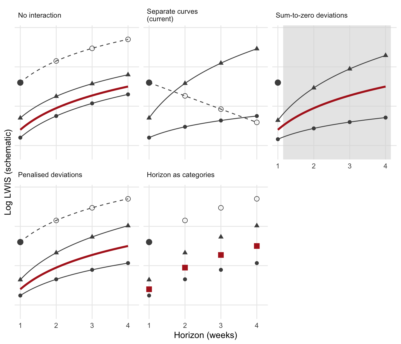
At the same time, we suspect that different models perform relatively better or worse than others at handling this horizon effect. However, some models forecast only one or two horizons, so have little or no information about their specific ability to handle different horizons.

Code
g <- \(x) 0.55 * log(x) / log(4)
shared <- \(x) 0.2 + g(x)
int_labels <- c("No interaction", "Separate curves (current)", "Sum-to-zero deviations",
                "Penalised deviations", "Horizon as categories")
lv <- \(d) mutate(d, p = factor(p, int_labels))
# models A and B: level and slope multiplier per specification
ab <- tibble(
  p = rep(int_labels, each = 2), model = rep(c("A", "B"), 5),
  level = c(-0.10, 0.15, -0.10, 0.15, -0.12, 0.12, -0.08, 0.12, -0.08, 0.12),
  slope = c(1, 1, 0.5, 1.6, 0.5, 1.5, 0.75, 1.25, 0.75, 1.25)
)
curve_ab <- crossing(ab, x = hf) |> mutate(y = 0.2 + level + slope * g(x))
point_ab <- crossing(ab, x = h) |> mutate(y = 0.2 + level + slope * g(x))
# model C: horizon 1 only
c_obs <- 0.8
pivot <- c(x = 2.45, y = shared(2.45))
c_fun <- list(
  `No interaction` = \(x) c_obs + g(x),
  `Separate curves (current)` = \(x) c_obs + (pivot[["y"]] - c_obs) * (x - 1) / (pivot[["x"]] - 1),
  `Penalised deviations` = \(x) c_obs + g(x),
  `Horizon as categories` = \(x) c_obs + g(x)
)
c_line <- imap_dfr(c_fun[1:3], \(f, p) tibble(p = p, x = hf, y = f(hf)))
c_pts <- imap_dfr(c_fun, \(f, p) tibble(p = p, x = h[-1], y = f(h[-1])))
ggplot(mapping = aes(x, y)) +
  geom_rect(data = lv(tibble(p = int_labels[3])), inherit.aes = FALSE,
            aes(xmin = 1.15, xmax = 4.15, ymin = -Inf, ymax = Inf),
            fill = "grey85", alpha = 0.6) +
  geom_line(data = lv(crossing(p = int_labels[c(1, 3, 4)], x = hf) |> mutate(y = shared(x))),
            colour = "firebrick", linewidth = 1.2) +
  geom_point(data = lv(tibble(p = int_labels[5], x = h, y = shared(h))),
             colour = "firebrick", size = 3, shape = 15) +
  geom_line(data = lv(filter(curve_ab, p != int_labels[5])), aes(group = model), colour = "grey30") +
  geom_point(data = lv(point_ab), aes(shape = model), colour = "grey30", size = 2) +
  geom_line(data = lv(c_line), colour = "grey30", linetype = "dashed") +
  geom_point(data = lv(c_pts), colour = "grey30", shape = 1, size = 2.5) +
  geom_point(data = lv(tibble(p = int_labels, x = 1, y = c_obs)), colour = "grey30", size = 3) +
  facet_wrap(~ p, ncol = 3, labeller = label_wrap_gen(25)) +
  scale_shape_manual(values = c(A = 16, B = 17), guide = "none") +
  scale_x_continuous(breaks = 1:4) +
  coord_cartesian(ylim = c(-0.1, 1.45)) +
  labs(x = "Horizon (weeks)", y = "Log LWIS (schematic)") +
  theme_minimal() +
  theme(axis.text.y = element_blank(), panel.grid.minor = element_blank(),
        strip.text = element_text(hjust = 0))
Schematic of how each specification treats three hypothetical models: two forecasting all horizons (filled, solid) and one forecasting only horizon 1 (large point). Open circles and dashed lines: the one-horizon model’s predictions at horizons it never forecast. Red: shared horizon curve. Separate curves: the one-horizon model’s level is absorbed into its unpenalised slope, so its line pivots through the average at the mean horizon of all forecasts and here falls with horizon. Sum-to-zero deviations: its slope is not identified by its own data (shaded). Sum-to-zero deviations + model level looks the same as sum-to-zero deviations. Schematic, not fitted.

Possible implementations

That suggests three requirements for the horizon and model terms:

  1. a shared horizon curve;
  2. an interaction with each model, allowing per-model deviations from the shared curve; models are penalised when they contribute less information
  3. each model’s level carried by only one term, as otherwise this gets arbitrarily split between different coefficients.
Specification Horizon and model terms 1. Shared curve 2. Deviations penalised 3. Level in one term
No interaction s(Model, bs="re") + s(Horizon, k=3) yes no deviations yes
Separate curves (current) s(Model, bs="re") + s(Horizon, by=Model, k=3) no no: linear part unpenalised no, for models with partial coverage
Sum-to-zero deviations s(Horizon, k=3) + s(Model, Horizon, k=3, bs="sz") yes no: intercept and slope per model unpenalised yes
Sum-to-zero deviations + model level s(Horizon, k=3) + s(Model, Horizon, k=3, bs="sz") + s(Model, bs="re") yes no no
Penalised deviations s(Horizon, k=3) + s(Horizon, Model, k=3, bs="fs") yes yes, one smoothing parameter yes
Penalised deviations, k = 4 s(Horizon, k=4) + s(Horizon, Model, k=4, bs="fs") yes yes, one smoothing parameter yes
Horizon as categories HorizonF + s(Model, bs="re") + s(Model, HorizonF, bs="re") yes, horizon unordered yes yes

Version: mgcv 1.9.4

The current model is s(Horizon, by=Model, k=3, bs="sz") .

  • This looks like it does the job, but in mgcv bs="sz" has no effect with by=.

  • With by= and no other factor terms within the smooth, mgcv defaults to a thin-plate basis smooth by model^[see smooth.construct.sz.smooth.spec]; so no shared term at all.

  • This results identical to s(Horizon, by=Model, k=3)

In sz and fs the per-model curves are not centred, so each carries its model’s level. Adding s(Model, bs="re") alongside them duplicates it.

  • Horizon as categories also meets all three requirements, but treats horizon as unordered; it keeps the model random effect used for reporting in the main analysis.

Only penalised deviations (fs) meets all three requirements with an ordered horizon, allowing each model its own variation on the shared curve.

A penalty \(\lambda \beta^\top S \beta\) is equivalent to a Gaussian prior \(\beta \sim N(0, (\lambda S)^-)\) (Wood 2017, section 5.8). \(S\) is rank deficient: along its null space, the unpenalised straight-line part of a thin-plate smooth, the prior has infinite variance, a flat improper prior (one that does not integrate to 1). An improper prior still gives a proper posterior if the data identify the parameter. In the current term, a model that forecast only horizon 1 does not identify its own slope, so that coefficient has an improper posterior; in frequentist terms it is unidentified and absorbs the model’s level. fs penalises every component of each model’s curve, giving each a proper prior.

The primary model has fitted separate curves per model since February 2025. Before that, horizon had a shared effect only, with no per-model variation.

Commit Date Horizon term Note
5476c90 2023-11-02 s(horizon_f, bs="fs"), horizon_f an ordered factor fs needs a numeric covariate; given only a factor, mgcv builds a plain random effect of horizon
497d87d 2024-04-12 Horizon, an ordered factor, as a fixed effect
55f0c4a 2025-02-06 s(Horizon, k=3, by=Model), numeric
d3c3299 2025-03-03 s(Horizon, k=3, by=Model, bs="sz") closes #57, which asked for an fs or sz spline centred against the model intercept
ab1316d 2026-01-04 univariate: s(Horizon, Model, bs="sz") a genuine sz term, univariate model only
c4a512c 2026-01-04 univariate: back to by=Model, k=3, bs="sz" “fix horizon as numeric not factor”

Verification

We fit a reduced model, LWIS ~ outcome + model + horizon, under each specification, with a Tweedie family and log link as in the primary analysis. Outcome (cases or deaths) is a fixed effect so that each model’s mix of outcomes does not enter its level. The fits show how each specification behaves; they are not used to choose between them.

Code
map_dfr(specs, \(x) tibble(
  Specification = arm_labels[[x$label]], edf = x$edf,
  `Deviance explained (%)` = 100 * x$dev_expl,
  `Tweedie p` = x$tweedie_p, Converged = x$converged,
  `Fit time (s)` = x$time_s
)) |>
  kable(digits = c(0, 1, 1, 2, 0, 0))
Specification edf Deviance explained (%) Tweedie p Converged Fit time (s)
No interaction 48.9 30.5 1.94 TRUE 61
Separate curves (current) 108.0 30.8 1.94 TRUE 94
Sum-to-zero deviations 101.3 30.8 1.94 TRUE 98
Sum-to-zero deviations + model level 101.3 30.8 1.94 TRUE 86
Penalised deviations 90.7 30.8 1.94 TRUE 86
Penalised deviations, k = 4 92.1 30.8 1.94 TRUE 88
Horizon as categories 131.1 30.8 1.94 TRUE 60

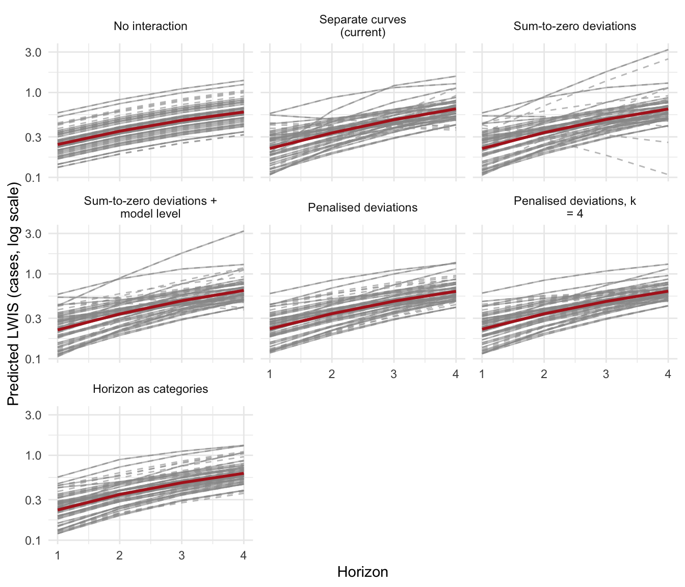
Predictions for models at horizons they never forecast are extrapolations; they are drawn dashed below and excluded from the comparisons.

Code
grid <- map_dfr(specs, \(x) mutate(x$grid, Arm = arm_labels[[x$label]])) |>
  mutate(Arm = factor(Arm, arm_labels)) |>
  left_join(coverage, by = "Model")
cases <- filter(grid, Epi_target == "Cases")
mean_curve <- cases |>
  filter(n_horizons == 4) |>
  group_by(Arm, Horizon) |>
  summarise(eta = mean(eta), .groups = "drop")
ggplot(cases, aes(Horizon, exp(eta), group = Model)) +
  geom_line(colour = "grey60", alpha = 0.6, linetype = "dashed") +
  geom_line(data = filter(cases, Horizon <= max_horizon),
            colour = "grey60", alpha = 0.6) +
  geom_line(data = mean_curve, aes(group = NULL),
            colour = "firebrick", linewidth = 1) +
  scale_y_log10() +
  facet_wrap(~Arm, labeller = label_wrap_gen(25)) +
  labs(y = "Predicted LWIS (cases, log scale)") +
  theme_minimal()

Predicted LWIS for cases by horizon. Grey: one line per model, dashed beyond the last horizon the model forecast. Red: geometric mean across models forecasting all four horizons.

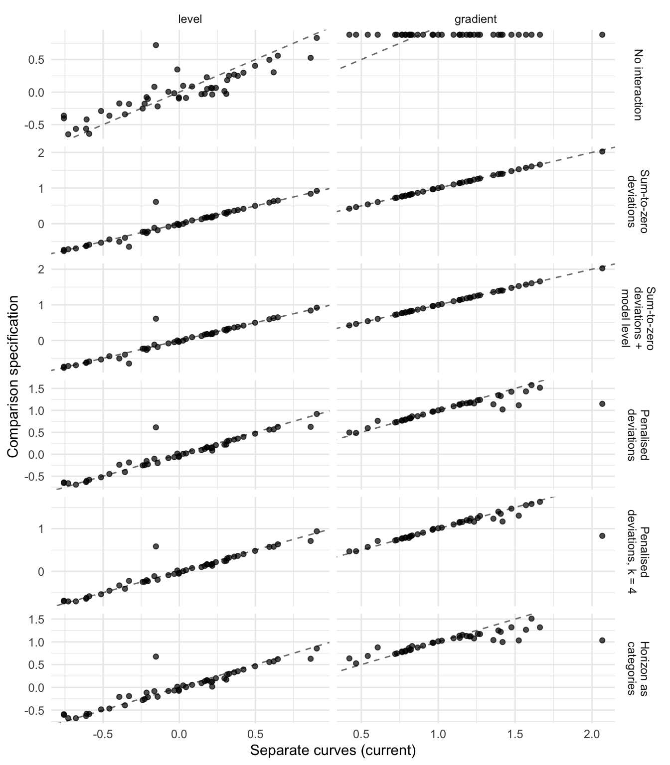
Each model is summarised by two quantities on the link scale, both independent of outcome: its level, the predicted log LWIS at horizon 1 (forecast by every model), centred on the mean across models; and its horizon gradient, the difference in predicted log LWIS between horizons 4 and 1, for models forecasting all four horizons. Level is the quantity closest to the individual model effect used for ranking in the main analysis.

Code
model_sum <- cases |>
  group_by(Arm, Model) |>
  summarise(level = eta[Horizon == 1],
            gradient = if_else(first(n_horizons) == 4,
                               eta[Horizon == 4] - eta[Horizon == 1], NA_real_),
            .groups = "drop_last") |>
  mutate(level = level - mean(level)) |>
  ungroup()
ref <- filter(model_sum, Arm == current) |>
  select(Model, ref_level = level, ref_gradient = gradient)
vs_ref <- model_sum |>
  filter(Arm != current) |>
  left_join(ref, by = "Model")
Code
vs_ref |>
  pivot_longer(c(level, gradient), names_to = "quantity") |>
  mutate(ref = if_else(quantity == "level", ref_level, ref_gradient),
         quantity = factor(quantity, c("level", "gradient"))) |>
  ggplot(aes(ref, value)) +
  geom_abline(linetype = "dashed", colour = "grey50") +
  geom_point(alpha = 0.7) +
  facet_grid(Arm ~ quantity, scales = "free", labeller = label_wrap_gen(18)) +
  labs(x = "Separate curves (current)", y = "Comparison specification") +
  theme_minimal()

Model level (left) and horizon gradient (right) under each specification, against the current specification. Dashed: identity.
Code
vs_ref |>
  group_by(Arm) |>
  summarise(
    `Spearman, level` = cor(level, ref_level, method = "spearman"),
    `Spearman, gradient` = cor(gradient, ref_gradient, method = "spearman",
                               use = "complete.obs"),
    `Models moving ≥10 places` = sum(abs(rank(level) - rank(ref_level)) >= 10),
    `Max level difference` = max(abs(level - ref_level))
  ) |>
  kable(digits = 2)
Arm Spearman, level Spearman, gradient Models moving ≥10 places Max level difference
No interaction 0.86 -0.19 5 0.87
Sum-to-zero deviations 0.96 1.00 1 0.76
Sum-to-zero deviations + model level 0.96 1.00 1 0.76
Penalised deviations 0.95 0.93 1 0.77
Penalised deviations, k = 4 0.95 0.92 1 0.74
Horizon as categories 0.94 0.89 1 0.83

Models with partial horizon coverage in the primary fit

In the current specification each model’s horizon curve is centred over the horizons of all forecasts, and the linear part of a thin-plate smooth is unpenalised. For a model that forecast only horizon 1, the curve’s value at horizon 1 is therefore unconstrained and absorbs the model’s whole level, leaving its model random effect at the prior. The primary fit shows this directly:

Code
primary <- readRDS(here("output", "log", "results.rds"))$effects
primary |>
  filter(group_var == "Model") |>
  inner_join(partial, by = c(group = "Model")) |>
  select(Model = group, Horizons = n_horizons, Forecasts = forecasts,
         model, value, lower = `lower_2.5`, upper = `upper_97.5`) |>
  pivot_wider(names_from = model, values_from = c(value, lower, upper)) |>
  select(Model, Horizons, Forecasts,
         Unadjusted = value_Unadjusted, Adjusted = value_Adjusted,
         `Adjusted lower` = lower_Adjusted, `Adjusted upper` = upper_Adjusted) |>
  arrange(Horizons, Model) |>
  kable(digits = 2)
Model Horizons Forecasts Unadjusted Adjusted Adjusted lower Adjusted upper
Imperial-DeCa 1 571 -0.87 0.31 0.16 0.46
Imperial-RtI0 1 571 -0.64 0.54 0.38 0.69
Imperial-sbkp 1 571 -0.73 0.45 0.30 0.60
SDSC_ISG-TrendModel 1 3500 0.10 0.38 0.25 0.51
UpgUmibUsi-MultiBayes 1 198 -1.14 -0.39 -0.58 -0.20
UC3M-EpiGraph 2 94 0.62 0.31 0.09 0.54
epiMOX-SUIHTER 2 267 -0.81 -0.35 -0.51 -0.19
UNED-PreCoV2 3 294 -0.12 -0.03 -0.17 0.12

Models forecasting only horizon 1 get an adjusted effect of exactly zero, with an interval equal to the fitted random-effect prior; those forecasting two horizons are shrunk close to zero. Their adjusted ranks, and so the before-and-after ranking comparison in the main text, reflect the specification rather than their performance. Specifications meeting requirement 2 (penalised deviations, horizon as categories) avoid this, since a model’s deviation at horizons it did not forecast is shrunk towards the shared curve rather than free.

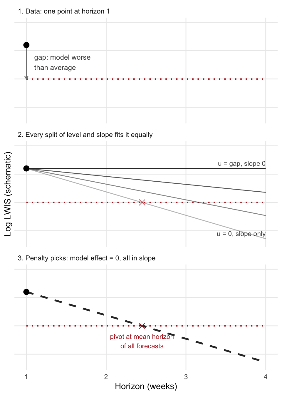
mgcv centres each model’s curve over the horizons of all forecasts in the data, so the crossing point is set by the other models’ horizon mix. With separate curves, a model’s prediction at horizon \(h\) is \(\beta_0 + u + a(h - \bar{h})\) plus a penalised bend, where \(u\) is the model’s random effect, \(a\) its own linear slope, and \(\bar{h}\) the horizon at which its curve crosses zero. \(\bar{h}\) is the mean horizon over all forecasts in the data, weighted by number of forecasts, not over the model’s own forecasts: 2.45 here, only slightly below the 2.5 of a balanced design, because the one-horizon models contribute few forecasts. For a model that forecast only horizon 1, the data fix only \(u + a(1 - \bar{h})\), the gap between its score and the average (panel 1). Every split of that gap between level and slope fits equally well (panel 2). \(u\) is penalised as a random effect but \(a\) is not, so the cheapest fit sets \(u = 0\) and puts the whole gap into the slope: a line through the observed point that crosses the average at \(\bar{h}\) (panel 3). The fit to the data is unaffected; the model’s effect in the ranking is lost.

Code
sc_b0 <- 0.5
sc_hbar <- 2.45
sc_obs <- 0.8
sc_hf <- seq(1, 4, length.out = 50)
sc_steps <- c("1. Data: one point at horizon 1",
              "2. Every split of level and slope fits it equally",
              "3. Penalty picks: model effect = 0, all in slope")
sc_lv <- \(d) mutate(d, p = factor(p, sc_steps))
sc_split <- tibble(u_share = c(1, 0.66, 0.33, 0),
                   label = c("u = gap, slope 0", "", "", "u = 0, slope only")) |>
  mutate(u = u_share * (sc_obs - sc_b0), a = (sc_obs - sc_b0 - u) / (1 - sc_hbar))
sc_lines <- crossing(sc_split, x = sc_hf) |>
  mutate(y = sc_b0 + u + a * (x - sc_hbar), p = sc_steps[2])
ggplot(mapping = aes(x, y)) +
  geom_line(data = sc_lv(crossing(p = sc_steps, x = sc_hf) |> mutate(y = sc_b0)),
            colour = "firebrick", linetype = "dotted", linewidth = 0.8) +
  geom_segment(data = sc_lv(tibble(p = sc_steps[1], x = 1, xend = 1, y = sc_b0, yend = sc_obs)),
               aes(xend = xend, yend = yend), colour = "grey50",
               arrow = arrow(length = unit(0.15, "cm"), ends = "both")) +
  geom_text(data = sc_lv(tibble(p = sc_steps[1], x = 1.1, y = (sc_b0 + sc_obs) / 2,
                                lab = "gap: model worse\nthan average")),
            aes(label = lab), hjust = 0, size = 3.2, colour = "grey30") +
  geom_line(data = sc_lv(sc_lines), aes(group = u_share, alpha = u_share), colour = "grey20") +
  geom_text(data = sc_lv(filter(sc_lines, x == 4, label != "")), aes(label = label),
            hjust = 1, vjust = -0.6, size = 3, colour = "grey30") +
  geom_line(data = sc_lv(filter(sc_lines, u_share == 0) |> mutate(p = sc_steps[3])),
            colour = "grey20", linewidth = 1.1, linetype = "dashed") +
  geom_point(data = sc_lv(tibble(p = sc_steps[2:3], x = sc_hbar, y = sc_b0)),
             shape = 4, size = 3, colour = "firebrick") +
  geom_text(data = sc_lv(tibble(p = sc_steps[3], x = sc_hbar, y = sc_b0 - 0.07,
                                lab = "pivot at mean horizon\nof all forecasts")),
            aes(label = lab), size = 3, colour = "firebrick", vjust = 1) +
  geom_point(data = sc_lv(tibble(p = sc_steps, x = 1, y = sc_obs)), size = 3) +
  facet_wrap(~p, ncol = 1) +
  scale_alpha_continuous(range = c(0.35, 1), guide = "none") +
  scale_x_continuous(breaks = 1:4) +
  coord_cartesian(ylim = c(0.15, 1)) +
  labs(x = "Horizon (weeks)", y = "Log LWIS (schematic)") +
  theme_minimal() +
  theme(axis.text.y = element_blank(), panel.grid.minor = element_blank(),
        strip.text = element_text(hjust = 0))
Separate curves, for a model forecasting only horizon 1 and scoring worse than average. Dotted red: average level. Cross: \(\bar{h}\), the mean horizon over all forecasts. Schematic.

Conclusion

Penalised deviations (fs) is the specification that matches the rationale: a shared horizon curve, with each model’s variation on it penalised towards that curve. The current specification has no shared curve and leaves each model’s linear deviation unpenalised, which is why the models forecasting only horizon 1 have adjusted effects at the prior.

Predicted levels at horizon 1 barely depend on the specification: against the current specification, rank correlations are 0.94 to 0.96 and one of 48 models moves ten or more places. The specification matters for how each model’s level is split between its model effect and its horizon curve, which is what the main analysis reports and ranks. Whether the change reaches the model structure effects and the ranking comparison needs a refit of the full model with penalised deviations.