Forecasting multiple data streams • EpiNow2

Background

The EpiNow2 package contains functionality to make forecasts for multiple data streams that represent different epidemiological outcomes. For example, it can be used to predict both the number of future cases (with symptoms) and severe cases (hospital admissions). This vignette demonstrates how to do this on an example simulated data set. For more information on the models used and the assumptions, look at the methods vignettes for estimate_infections and estimate_secondary.

Setup

We first load the EpiNow2 package. We also load data.table and ggplot2 which we’ll use later for data manipulation and plotting. Lastly, we set a seed for reproducibility.

library(EpiNow2)
#> 
#> Attaching package: 'EpiNow2'
#> The following object is masked from 'package:stats':
#> 
#>     Gamma
library(data.table)
library(ggplot2)
set.seed(6789)

To speed up compuation you can set the number of cores to use. We will want to run 4 MCMC chains in parallel so if this is available it would make sense to set:

options(mc.cores = 4)

If we had fewer than 4 available or wanted to run fewer than 4 chains (at the expense of some robustness), or had fewer than 4 computing cores available we could set it to that. To find out the number of cores available one can use the detectCores function from the parallel package.

Data

We first simulate a data set that we will use as an example.

Simulation code

cases <- example_confirmed[1:60]

We then generate another data set of hospitalisations, assuming that 10% of confirmed cases become hospitalised with a delay from case confirmation that is given by a lognormal distribution with mean of 7 days and standard deviation of 3 days.

admission_delay <- LogNormal(mean = 7, sd = 3)
admission_scale <- Fixed(0.1)

We use the simulate_secondary function to generate a time series of hospitalisations

## first, rename the column to what is expected by `simulate_secondary`
primary <- cases[, list(date, primary = confirm)]
## generate hospitalisation data
hosp <- simulate_secondary(
  primary,
  delays = delay_opts(admission_delay),
  obs = obs_opts(family = "poisson", scale = admission_scale)
)
#> ℹ Unconstrained distributon passed as a delay.
#> ℹ Constraining with default CDF cutoff 0.001.
#> ℹ To silence this message, specify delay distributions with `max` or
#>   `default_cdf_cutoff`.

Using this we then create a combined data set:

df <- merge(primary, hosp, by = "date")
setnames(
  df,
  c("date", "primary", "secondary"),
  c("date", "cases", "hospitalisations")
)

The simulated data set looks like this:

head(df)
#> Key: <date>
#>          date cases hospitalisations
#>        <Date> <num>            <num>
#> 1: 2020-02-22    14                0
#> 2: 2020-02-23    62                0
#> 3: 2020-02-24    53                0
#> 4: 2020-02-25    97                0
#> 5: 2020-02-26    93                1
#> 6: 2020-02-27    78                1

df_long <- melt(df, id.vars = "date")
ggplot(df_long, aes(x = date, y = value, colour = variable)) +
  geom_line() +
  xlab("Value") + ylab("Date") +
  theme_bw() +
  theme(legend.position = "bottom")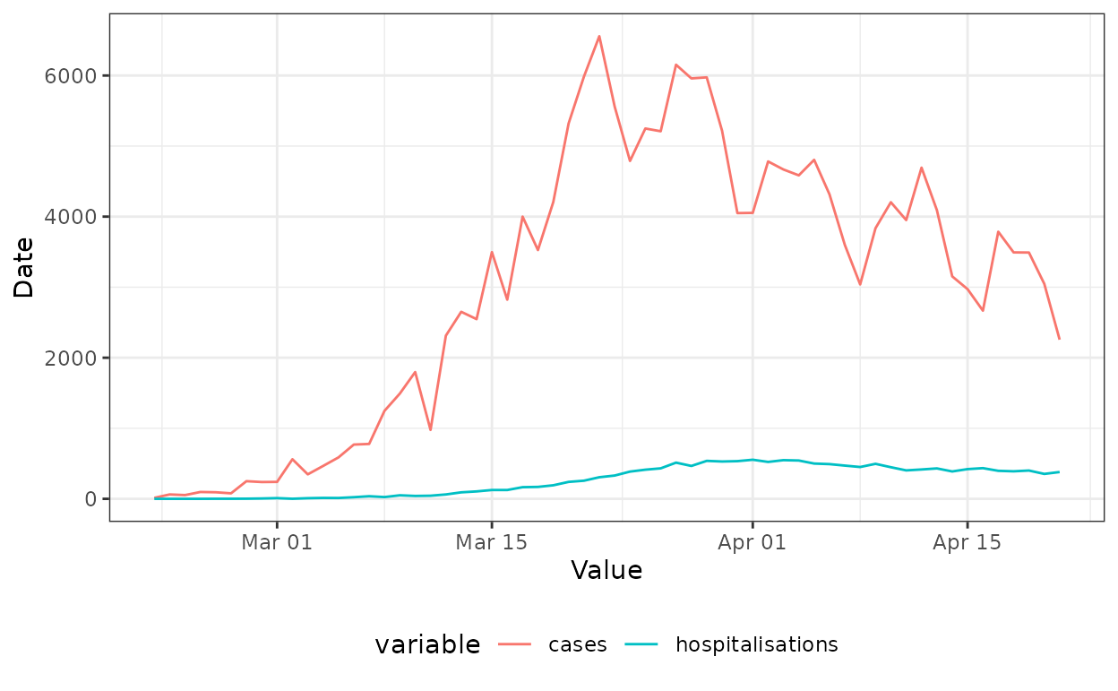

Estimating infections

We first use one of the two data streams to estimate the number of infections and make a forecast. Usually this would be done on the outcome that is closest to infection, in our case the number of confirmed cases. In order to do so, we would usually specify a number generation time and any delays to the initial report. This should be done based on insight on the disease and reporting set up. Here we use some example parameters, the same as in the workflow vignette:

generation_time <- Gamma(
  shape = Normal(9, 2.5), rate = Normal(3, 1.4), max = 10
)
incubation_period <- LogNormal(
  meanlog = Normal(1.6, 0.05),
  sdlog = Normal(0.5, 0.05),
  max = 14
)
reporting_delay <- LogNormal(meanlog = 0.5, sdlog = 0.5, max = 10)
combined_delays <- incubation_period + reporting_delay

We then estimate infections and produce a 2-week forecast.

est <- estimate_infections(
  df[, list(date, confirm = cases)],
  generation_time = gt_opts(generation_time),
  delay = delay_opts(combined_delays),
  forecast = forecast_opts(horizon = 14)
)

Estimating secondary scaling and delay

We next use our data sets of cases and admissions to estimate the delay and scaling between the two (both of which assumed to be constant over time). This is done using the estimate_secondary() function.

sec <- estimate_secondary(
  df[, list(date, primary = cases, secondary = hospitalisations)],
  obs = obs_opts(scale = Normal(0, 1))
)

Forecasting secondary outcomes

We can now combine our case forecast with the estimated delay and scaling to make forecasts of the number of hospitalisations. In order to do so we use the forecast_secondary function.

forecast <- forecast_secondary(
  sec, est
)

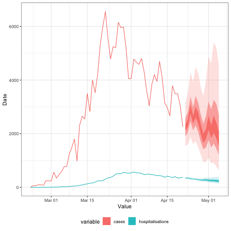
We can now combine all our forecasts into one plot:

case_forecast <- est$summarised[
  variable == "reported_cases" & type == "forecast"
][, variable := "cases"]
admissions_forecast <- forecast$predictions[
  is.na(secondary)
][, variable := "hospitalisations"]
forecasts <- rbindlist(list(case_forecast, admissions_forecast), fill = TRUE)

ggplot(df_long, aes(x = date, colour = variable, fill = variable)) +
  geom_line(aes(y = value)) +
  geom_ribbon(
    data = forecasts, aes(ymin = lower_20, ymax = upper_20), alpha = 0.8,
    colour = NA
  ) +
  geom_ribbon(
    data = forecasts, aes(ymin = lower_50, ymax = upper_50), alpha = 0.5,
    colour = NA
  ) +
  geom_ribbon(
    data = forecasts, aes(ymin = lower_90, ymax = upper_90), alpha = 0.2,
    colour = NA
  ) +
  xlab("Value") + ylab("Date") +
  theme_bw() +
  theme(legend.position = "bottom")