The EpiNow2 package contains functionality to run
estimate_infections() in production mode, i.e. with full
logging and saving all relevant outputs and plots to dedicated folders
in the hard drive. This is done with the epinow() function,
that takes the same options as estimate_infections() with
some additional options that determine, for example, where output gets
stored and what output exactly. The function can be a useful option
when, e.g., running the model daily with updated data on a
high-performance computing server to feed into a dashboard. For more
detail on the various model options available, see the Examples vignette, for more
on the general modelling approach the Workflow, and for
theoretical background the Model
definitions vignette
Running the model on a single region
To run the model in production mode for a single region, set the
parameters up in the same way as for estimate_infections()
(see the Workflow
vignette). Here we use the example delay and generation time
distributions that come with the package. This should be replaced with
parameters relevant to the system that is being studied.
library("EpiNow2")
#>
#> Attaching package: 'EpiNow2'
#> The following object is masked from 'package:stats':
#>
#>     Gamma
options(mc.cores = 4)
reported_cases <- example_confirmed[1:60]
reporting_delay <- LogNormal(mean = 2, sd = 1, max = 10)
delay <- example_incubation_period + reporting_delay
rt_prior <- LogNormal(mean = 2, sd = 1)
We can then run the epinow() function with the same
arguments as estimate_infections().
res <- epinow(reported_cases,
  generation_time = gt_opts(example_generation_time),
  delays = delay_opts(delay),
  rt = rt_opts(prior = rt_prior),
  logs = NULL
)
plot(res)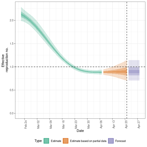
By default, logging messages are printed to the console indicating
the progress of the model fitting and where log files can be found. Here
we have set logs = NULL to suppress these messages. If you
want summarised results and plots to be written out where they can be
accessed later you can use the target_folder argument.
Running the model simultaneously on multiple regions
The package also contains functionality to conduct inference
contemporaneously (if separately) in production mode on multiple time
series, e.g. to run the model on multiple regions. This is done with the
regional_epinow() function.
Say, for example, we construct a dataset containing two regions,
testland and realland (in this simple example
both containing the same case data).
cases <- example_confirmed[1:60]
cases <- data.table::rbindlist(list(
  data.table::copy(cases)[, region := "testland"],
  cases[, region := "realland"]
 ))
To then run this on multiple regions using the default options above, we could use
region_rt <- regional_epinow(
data = cases,
generation_time = gt_opts(example_generation_time),
delays = delay_opts(delay),
rt = rt_opts(prior = rt_prior),
logs = NULL
)
## summary
region_rt$summary$summarised_results$table
#> Region New infections per day Expected change in reports
#> <char> <char> <fctr>
#> 1: realland 2265 (1417 -- 3779) Likely decreasing
#> 2: testland 2223 (1370 -- 3711) Likely decreasing
#> Effective reproduction no. Rate of growth
#> <char> <char>
#> 1: 0.9 (0.73 -- 1.1) -0.028 (-0.09 -- 0.04)
#> 2: 0.89 (0.71 -- 1.1) -0.031 (-0.092 -- 0.039)
#> Doubling/halving time (days)
#> <char>
#> 1: -25 (17 -- -7.7)
#> 2: -23 (18 -- -7.5)
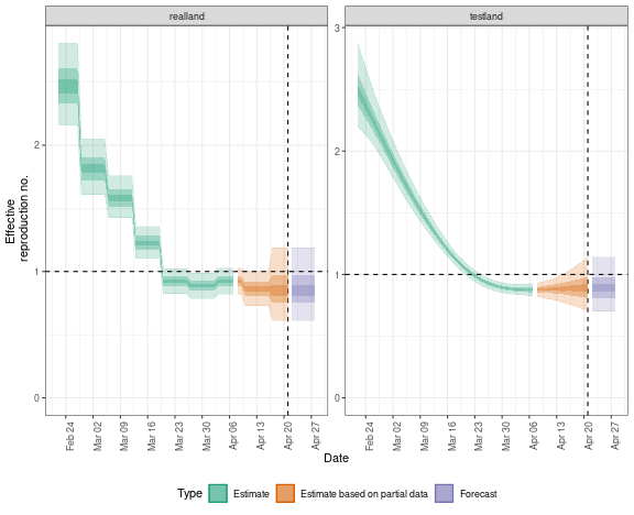
## plot
region_rt$summary$plots$R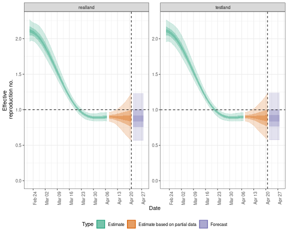
If instead, we wanted to use the Gaussian Process for
testland and a weekly random walk for realland
we could specify these separately using the opts_list()
function from the package and modifyList() from
R.
gp <- opts_list(gp_opts(), cases)
gp <- modifyList(gp, list(realland = NULL), keep.null = TRUE)
rt <- opts_list(rt_opts(), cases, realland = rt_opts(rw = 7))
region_separate_rt <- regional_epinow(
  data = cases,
  generation_time = gt_opts(example_generation_time),
  delays = delay_opts(delay),
  rt = rt, gp = gp,
  logs = NULL
)
## summary
region_separate_rt$summary$summarised_results$table
#>      Region New infections per day Expected change in reports
#>      <char>                 <char>                     <fctr>
#> 1: realland    1993 (1057 -- 3827)          Likely decreasing
#> 2: testland      1984 (27 -- 3481)          Likely decreasing
#>    Effective reproduction no.          Rate of growth
#>                        <char>                  <char>
#> 1:         0.85 (0.61 -- 1.2) -0.042 (-0.11 -- 0.037)
#> 2:         0.95 (0.73 -- 1.9) -0.01 (-0.087 -- 0.042)
#>    Doubling/halving time (days)
#>                          <char>
#> 1:             -17 (19 -- -6.2)
#> 2:             -67 (16 -- -7.9)
## plot
region_separate_rt$summary$plots$R