Quick start
In the following section we give an overview of the simple use case
for epinow() and regional_epinow().
The first step to using the package is to load it as follows.
Reporting delays, incubation period and generation time
Distributions can be supplied in two ways. First, one can supply
delay data to estimate_delay(), where a subsampled
bootstrapped lognormal will be fit to account for uncertainty in the
observed data without being biased by changes in incidence (see
?EpiNow2::estimate_delay()).
Second, one can specify predetermined delays with uncertainty using
the distribution functions such as Gamma or
LogNormal. An arbitrary number of delay distributions are
supported in dist_spec() with a common use case being an
incubation period followed by a reporting delay. For more information on
specifying distributions see ?EpiNow2::Distributions or the
delays vignette.
For example if data on the delay between onset and infection was
available we could fit a distribution to it, using
estimate_delay(), with appropriate uncertainty as follows
(note this is a synthetic example),
reporting_delay <- estimate_delay(
  rlnorm(1000, log(2), 1),
  max_value = 14, bootstraps = 1
)
If data was not available we could instead specify an informed
estimate of the likely delay using the distribution functions
Gamma or LogNormal. To demonstrate, we choose
a lognormal distribution with mean 2, standard deviation 1 and a maximum
of 10. This is just an example and unlikely to apply in any
particular use case.
reporting_delay <- LogNormal(mean = 2, sd = 1, max = 10)
reporting_delay
#> - lognormal distribution (max: 10):
#>   meanlog:
#>     0.58
#>   sdlog:
#>     0.47
For the rest of this vignette, we will use inbuilt example literature estimates for the incubation period and generation time of Covid-19 (see here for the code that generates these estimates). These distributions are unlikely to be applicable for your use case. We strongly recommend investigating what might be the best distributions to use in any given use case.
example_generation_time
#> - gamma distribution (max: 14):
#>   shape:
#>     - normal distribution:
#>       mean:
#>         1.4
#>       sd:
#>         0.48
#>   rate:
#>     - normal distribution:
#>       mean:
#>         0.38
#>       sd:
#>         0.25
example_incubation_period
#> - lognormal distribution (max: 14):
#>   meanlog:
#>     - normal distribution:
#>       mean:
#>         1.6
#>       sd:
#>         0.064
#>   sdlog:
#>     - normal distribution:
#>       mean:
#>         0.42
#>       sd:
#>         0.069
Users can also pass a non-parametric delay distribution vector using
the NonParametric option for both the generation interval
and reporting delays. It is important to note that if doing so, both
delay distributions are 0-indexed, meaning the first element corresponds
to the probability mass at day 0 of an individual’s infection. Because
the discretised renewal equation doesn’t support mass on day 0, the
generation interval should be passed in as a 0-indexed vector with a
mass of zero on day 0.
example_non_parametric_gi <-  NonParametric(pmf = c(0, 0.3, 0.5, 0.2))

example_non_parametric_delay <- NonParametric(pmf = c(0.01, 0.1, 0.5, 0.3, 0.09))
These distributions are passed to downstream functions in the same way that the parametric distributions are.
Now, to the functions.
epinow()
This function represents the core functionality of the package and includes results reporting, plotting, and optional saving. It requires a data frame of cases by date of report and the distributions defined above.
Load example case data from EpiNow2.
reported_cases <- example_confirmed[1:60]
head(reported_cases)
#>          date confirm
#>        <Date>   <num>
#> 1: 2020-02-22      14
#> 2: 2020-02-23      62
#> 3: 2020-02-24      53
#> 4: 2020-02-25      97
#> 5: 2020-02-26      93
#> 6: 2020-02-27      78
Estimate cases by date of infection, the time-varying reproduction
number, the rate of growth, and forecast these estimates into the future
by 7 days. Summarise the posterior and return a summary table and plots
for reporting purposes. If a target_folder is supplied
results can be internally saved (with the option to also turn off
explicit returning of results).
estimates <- epinow(
  data = reported_cases,
  generation_time = gt_opts(example_generation_time),
  delays = delay_opts(example_incubation_period + reporting_delay),
  rt = rt_opts(prior = LogNormal(mean = 2, sd = 0.2)),
  stan = stan_opts(cores = 4),
  verbose = interactive()
)
names(estimates)
#> [1] "fit"          "args"         "observations" "timing"
The default model uses a Gaussian process to estimate time-varying transmission, which provides flexible estimates but can take several minutes to run. If speed is a priority, there are several alternatives:
- Use a weekly random walk instead of the Gaussian process
(
rt = rt_opts(..., rw = 7)withgp = NULL), as shown in theregional_epinow()example below. - Use variational inference for fast but unreliable approximate
results (
stan = stan_opts(method = "vb")). - Reduce the accuracy of the Gaussian process approximation (see
?gp_opts).
For examples of different model configurations, see the estimate_infections_options vignette.
Both summary measures and posterior samples are returned for all
parameters in an easily explored format which can be accessed using
summary. The default is to return a summary table of
estimates for key parameters at the latest date partially supported by
data.
| measure | estimate |
|---|---|
| New infections per day | 2240 (1363 – 3709) |
| Expected change in reports | Likely decreasing |
| Effective reproduction no. | 0.89 (0.72 – 1.1) |
| Rate of growth | -0.03 (-0.096 – 0.038) |
| Doubling/halving time (days) | -23 (18 – -7.2) |
Summarised parameter estimates can also easily be returned, either filtered for a single parameter or for all parameters.
head(summary(estimates, type = "parameters", params = "R"))
#>          date variable strat     type   median     mean         sd lower_90
#>        <Date>   <char> <int>   <char>    <num>    <num>      <num>    <num>
#> 1: 2020-02-22        R    NA estimate 2.178490 2.184456 0.12007169 1.993521
#> 2: 2020-02-23        R    NA estimate 2.143038 2.146818 0.10919319 1.972582
#> 3: 2020-02-24        R    NA estimate 2.104298 2.107843 0.10069813 1.947632
#> 4: 2020-02-25        R    NA estimate 2.062887 2.067720 0.09427498 1.918777
#> 5: 2020-02-26        R    NA estimate 2.022027 2.026632 0.08946219 1.886428
#> 6: 2020-02-27        R    NA estimate 1.980695 1.984750 0.08574980 1.851349
#>    lower_50 lower_20 upper_20 upper_50 upper_90
#>       <num>    <num>    <num>    <num>    <num>
#> 1: 2.104145 2.150307 2.208533 2.262534 2.385199
#> 2: 2.073533 2.115388 2.167645 2.217938 2.330660
#> 3: 2.040771 2.078324 2.128667 2.170718 2.280794
#> 4: 2.001783 2.041288 2.085802 2.126371 2.227861
#> 5: 1.963473 2.000645 2.045253 2.083873 2.180490
#> 6: 1.924749 1.959991 2.003451 2.040541 2.132498
Reported cases can be extracted using get_predictions()
which returns summarised estimates by default.
head(get_predictions(estimates))
#>          date median     mean        sd lower_90 lower_50 lower_20 upper_20
#>        <Date>  <num>    <num>     <num>    <num>    <num>    <num>    <num>
#> 1: 2020-02-22     35  35.9840  9.774483       21       29     33.0       38
#> 2: 2020-02-23     53  53.5585 13.729998       33       44     49.0       56
#> 3: 2020-02-24     64  65.2305 15.386804       42       55     60.6       68
#> 4: 2020-02-25     72  73.1890 16.513589       48       61     68.0       76
#> 5: 2020-02-26     82  83.2085 18.383280       56       70     78.0       87
#> 6: 2020-02-27    119 120.7925 24.347502       84      104    113.0      125
#>    upper_50 upper_90
#>       <num>    <num>
#> 1:       42       53
#> 2:       62       78
#> 3:       74       93
#> 4:       84      103
#> 5:       94      116
#> 6:      137      162
A range of plots are returned (with the single summary plot shown
below). These plots can also be generated using the following
plot method.
plot(estimates)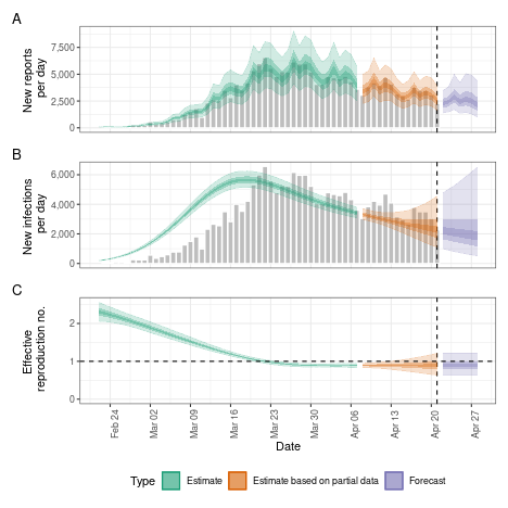
regional_epinow()
The regional_epinow() function runs the
epinow() function across multiple regions in an efficient
manner.
Define cases in multiple regions delineated by the region variable.
reported_cases <- data.table::rbindlist(list(
  data.table::copy(reported_cases)[, region := "testland"],
  reported_cases[, region := "realland"]
))
head(reported_cases)
#>          date confirm   region
#>        <Date>   <num>   <char>
#> 1: 2020-02-22      14 testland
#> 2: 2020-02-23      62 testland
#> 3: 2020-02-24      53 testland
#> 4: 2020-02-25      97 testland
#> 5: 2020-02-26      93 testland
#> 6: 2020-02-27      78 testland
Calling regional_epinow() runs the epinow()
on each region in turn (or in parallel depending on the settings used).
Here we switch to using a weekly random walk rather than the full
Gaussian process model giving us piecewise constant estimates by week.
We also assign “testland” a different ascertainment of 50%, using the
opts_list() function, which is used to assign
region-specific settings.
obs <- opts_list(
  obs_opts(),
  reported_cases,
  testland = obs_opts(scale = Fixed(0.5))
)

estimates <- regional_epinow(
  data = reported_cases,
  generation_time = gt_opts(example_generation_time),
  delays = delay_opts(example_incubation_period + reporting_delay),
  rt = rt_opts(prior = LogNormal(mean = 2, sd = 0.2), rw = 7),
  obs = obs,
  gp = NULL,
  stan = stan_opts(cores = 4, warmup = 250, samples = 1000),
  logs = NULL
)
Results from each region are stored in a regional list
with across region summary measures and plots stored in a
summary list. All results can be set to be internally saved
by setting the target_folder and summary_dir
arguments. Each region can be estimated in parallel using the
future package (when in most scenarios cores
should be set to 1). For routine use each MCMC chain can also be run in
parallel (with future = TRUE) with a time out
(max_execution_time) allowing for partial results to be
returned if a subset of chains is running longer than expected. See the
documentation for the {future} package
for details on nested futures.
Summary measures that are returned include a table formatted for reporting (along with raw results for further processing).
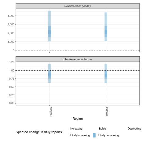
knitr::kable(estimates$summary$summarised_results$table)| Region | New infections per day | Expected change in reports | Effective reproduction no. | Rate of growth | Doubling/halving time (days) |
|---|---|---|---|---|---|
| realland | 1987 (1029 – 4104) | Likely decreasing | 0.84 (0.61 – 1.2) | -0.044 (-0.11 – 0.044) | -16 (16 – -6) |
| testland | 3965 (2135 – 7945) | Likely decreasing | 0.85 (0.62 – 1.2) | -0.043 (-0.11 – 0.038) | -16 (18 – -6.2) |
A range of plots are again returned (with the single summary plot shown below).
estimates$summary$summary_plot