Real-time Rt Estimation, Forecasting and Reporting

This function wraps the functionality of estimate_infections() in order to estimate Rt and cases by date of infection and forecast these infections into the future. In addition to the functionality of estimate_infections() it produces additional summary output useful for reporting results and interpreting them as well as error catching and reporting, making it particularly useful for production use e.g. running at set intervals on a dedicated server.

Usage

epinow(
  reported_cases,
  generation_time = generation_time_opts(),
  delays = delay_opts(),
  truncation = trunc_opts(),
  rt = rt_opts(),
  backcalc = backcalc_opts(),
  gp = gp_opts(),
  obs = obs_opts(),
  stan = stan_opts(),
  horizon = 7,
  CrIs = c(0.2, 0.5, 0.9),
  filter_leading_zeros = TRUE,
  zero_threshold = Inf,
  return_output = FALSE,
  output = c("samples", "plots", "latest", "fit", "timing"),
  plot_args = list(),
  target_folder = NULL,
  target_date,
  logs = tempdir(),
  id = "epinow",
  verbose = interactive()
)

Arguments

reported_cases: A <data.frame> of confirmed cases (confirm) by date (date). confirm must be numeric and date must be in date format.
generation_time: A call to generation_time_opts() defining the generation time distribution used. For backwards compatibility a list of summary parameters can also be passed.
delays: A call to delay_opts() defining delay distributions and options. See the documentation of delay_opts() and the examples below for details.
truncation: A call to trunc_opts() defining the truncation of observed data. Defaults to trunc_opts(). See estimate_truncation() for an approach to estimating truncation from data.
rt: A list of options as generated by rt_opts() defining Rt estimation. Defaults to rt_opts(). Set to NULL to switch to using back calculation rather than generating infections using Rt.
backcalc: A list of options as generated by backcalc_opts() to define the back calculation. Defaults to backcalc_opts().
gp: A list of options as generated by gp_opts() to define the Gaussian process. Defaults to gp_opts(). Set to NULL to disable the Gaussian process.
obs: A list of options as generated by obs_opts() defining the observation model. Defaults to obs_opts().
stan: A list of stan options as generated by stan_opts(). Defaults to stan_opts(). Can be used to override data, init, and verbose settings if desired.
horizon: Numeric, defaults to 7. Number of days into the future to forecast.
CrIs: Numeric vector of credible intervals to calculate.
filter_leading_zeros: Logical, defaults to TRUE. Should zeros at the start of the time series be filtered out.
zero_threshold: Numeric defaults to Inf. Indicates if detected zero cases are meaningful by using a threshold number of cases based on the 7-day average. If the average is above this threshold then the zero is replaced using fill.
return_output: Logical, defaults to FALSE. Should output be returned, this automatically updates to TRUE if no directory for saving is specified.
output: A character vector of optional output to return. Supported options are samples ("samples"), plots ("plots"), the run time ("timing"), copying the dated folder into a latest folder (if target_folder is not null, set using "latest"), and the stan fit ("fit"). The default is to return all options.
plot_args: A list of optional arguments passed to plot.epinow().
target_folder: Character string specifying where to save results (will create if not present).
target_date: Date, defaults to maximum found in the data if not specified.
logs: Character path indicating the target folder in which to store log information. Defaults to the temporary directory if not specified. Default logging can be disabled if logs is set to NULL. If specifying a custom logging setup then the code for setup_default_logging() and the setup_logging() function are a sensible place to start.
id: A character string used to assign logging information on error. Used by regional_epinow() to assign errors to regions. Alter the default to run with error catching.
verbose: Logical, defaults to TRUE when used interactively and otherwise FALSE. Should verbose debug progress messages be printed. Corresponds to the "DEBUG" level from futile.logger. See setup_logging for more detailed logging options.

Value

A list of output from estimate_infections with additional elements summarising results and reporting errors if they have occurred.

Examples

# \donttest{
# set number of cores to use
old_opts <- options()
options(mc.cores = ifelse(interactive(), 4, 1))

# set an example generation time. In practice this should use an estimate
# from the literature or be estimated from data
generation_time <- Gamma(
  shape = Normal(1.3, 0.3),
  rate = Normal(0.37, 0.09),
  max = 14
)
# set an example incubation period. In practice this should use an estimate
# from the literature or be estimated from data
incubation_period <- LogNormal(
   meanlog = Normal(1.6, 0.06),
   sdlog = Normal(0.4, 0.07),
   max = 14
)
# set an example reporting delay. In practice this should use an estimate
# from the literature or be estimated from data
reporting_delay <- LogNormal(mean = 2, sd = 1, max = 10)

# example case data
reported_cases <- example_confirmed[1:40]

# estimate Rt and nowcast/forecast cases by date of infection
out <- epinow(
  reported_cases = reported_cases,
  generation_time = generation_time_opts(generation_time),
  rt = rt_opts(prior = list(mean = 2, sd = 0.1)),
  delays = delay_opts(incubation_period + reporting_delay)
)
#> Logging threshold set at INFO for the EpiNow2 logger
#> Writing EpiNow2 logs to the console and: /tmp/Rtmpv9ckcg/regional-epinow/2020-04-01.log
#> Logging threshold set at INFO for the EpiNow2.epinow logger
#> Writing EpiNow2.epinow logs to the console and: /tmp/Rtmpv9ckcg/epinow/2020-04-01.log
#> WARN [2024-04-19 08:09:30] epinow: There were 5 divergent transitions after warmup. See
#> https://mc-stan.org/misc/warnings.html#divergent-transitions-after-warmup
#> to find out why this is a problem and how to eliminate them. - 
#> WARN [2024-04-19 08:09:30] epinow: Examine the pairs() plot to diagnose sampling problems
#>  - 
# summary of the latest estimates
summary(out)
#>                             measure                estimate
#>                              <char>                  <char>
#> 1:           New infections per day     3041 (1146 -- 8062)
#> 2: Expected change in daily reports       Likely decreasing
#> 3:       Effective reproduction no.      0.76 (0.46 -- 1.2)
#> 4:                   Rate of growth -0.079 (-0.21 -- 0.065)
#> 5:     Doubling/halving time (days)       -8.8 (11 -- -3.3)
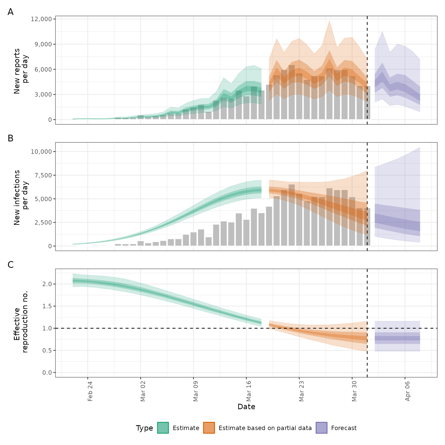
# plot estimates
plot(out)


# summary of R estimates
summary(out, type = "parameters", params = "R")
#>           date variable  strat                           type    median
#>         <Date>   <char> <char>                         <char>     <num>
#>  1: 2020-02-22        R   <NA>                       estimate 2.0761619
#>  2: 2020-02-23        R   <NA>                       estimate 2.0690354
#>  3: 2020-02-24        R   <NA>                       estimate 2.0583705
#>  4: 2020-02-25        R   <NA>                       estimate 2.0419396
#>  5: 2020-02-26        R   <NA>                       estimate 2.0213950
#>  6: 2020-02-27        R   <NA>                       estimate 1.9965881
#>  7: 2020-02-28        R   <NA>                       estimate 1.9685325
#>  8: 2020-02-29        R   <NA>                       estimate 1.9371994
#>  9: 2020-03-01        R   <NA>                       estimate 1.9025202
#> 10: 2020-03-02        R   <NA>                       estimate 1.8649238
#> 11: 2020-03-03        R   <NA>                       estimate 1.8249665
#> 12: 2020-03-04        R   <NA>                       estimate 1.7821740
#> 13: 2020-03-05        R   <NA>                       estimate 1.7378490
#> 14: 2020-03-06        R   <NA>                       estimate 1.6922530
#> 15: 2020-03-07        R   <NA>                       estimate 1.6452452
#> 16: 2020-03-08        R   <NA>                       estimate 1.5966458
#> 17: 2020-03-09        R   <NA>                       estimate 1.5471827
#> 18: 2020-03-10        R   <NA>                       estimate 1.4968382
#> 19: 2020-03-11        R   <NA>                       estimate 1.4478656
#> 20: 2020-03-12        R   <NA>                       estimate 1.3986076
#> 21: 2020-03-13        R   <NA>                       estimate 1.3502342
#> 22: 2020-03-14        R   <NA>                       estimate 1.3018548
#> 23: 2020-03-15        R   <NA>                       estimate 1.2554572
#> 24: 2020-03-16        R   <NA>                       estimate 1.2103429
#> 25: 2020-03-17        R   <NA>                       estimate 1.1655709
#> 26: 2020-03-18        R   <NA>                       estimate 1.1235316
#> 27: 2020-03-19        R   <NA> estimate based on partial data 1.0829845
#> 28: 2020-03-20        R   <NA> estimate based on partial data 1.0440472
#> 29: 2020-03-21        R   <NA> estimate based on partial data 1.0083385
#> 30: 2020-03-22        R   <NA> estimate based on partial data 0.9746836
#> 31: 2020-03-23        R   <NA> estimate based on partial data 0.9443066
#> 32: 2020-03-24        R   <NA> estimate based on partial data 0.9163639
#> 33: 2020-03-25        R   <NA> estimate based on partial data 0.8902631
#> 34: 2020-03-26        R   <NA> estimate based on partial data 0.8652876
#> 35: 2020-03-27        R   <NA> estimate based on partial data 0.8430470
#> 36: 2020-03-28        R   <NA> estimate based on partial data 0.8228334
#> 37: 2020-03-29        R   <NA> estimate based on partial data 0.8046003
#> 38: 2020-03-30        R   <NA> estimate based on partial data 0.7864915
#> 39: 2020-03-31        R   <NA> estimate based on partial data 0.7709292
#> 40: 2020-04-01        R   <NA> estimate based on partial data 0.7584099
#> 41: 2020-04-02        R   <NA>                       forecast 0.7584099
#> 42: 2020-04-03        R   <NA>                       forecast 0.7584099
#> 43: 2020-04-04        R   <NA>                       forecast 0.7584099
#> 44: 2020-04-05        R   <NA>                       forecast 0.7584099
#> 45: 2020-04-06        R   <NA>                       forecast 0.7584099
#> 46: 2020-04-07        R   <NA>                       forecast 0.7584099
#> 47: 2020-04-08        R   <NA>                       forecast 0.7584099
#>           date variable  strat                           type    median
#>          mean         sd  lower_90  lower_50  lower_20  upper_20  upper_50
#>         <num>      <num>     <num>     <num>     <num>     <num>     <num>
#>  1: 2.0763844 0.09229418 1.9311083 2.0139889 2.0511310 2.0999364 2.1366699
#>  2: 2.0686706 0.08220381 1.9384205 2.0120663 2.0487773 2.0889618 2.1201795
#>  3: 2.0576555 0.07926444 1.9294181 2.0029192 2.0384159 2.0764582 2.1073591
#>  4: 2.0428809 0.08065863 1.9135584 1.9887632 2.0223946 2.0591774 2.0922161
#>  5: 2.0240454 0.08328625 1.8930306 1.9718401 2.0017956 2.0397579 2.0733980
#>  6: 2.0010244 0.08517426 1.8655561 1.9465471 1.9767518 2.0164674 2.0521900
#>  7: 1.9738678 0.08556334 1.8357488 1.9176054 1.9497532 1.9890617 2.0277918
#>  8: 1.9427773 0.08448941 1.8082046 1.8892967 1.9179452 1.9577456 1.9968913
#>  9: 1.9080700 0.08236223 1.7777581 1.8555034 1.8835417 1.9222324 1.9597181
#> 10: 1.8701372 0.07965342 1.7440212 1.8181679 1.8462286 1.8846914 1.9199808
#> 11: 1.8294058 0.07671569 1.7079648 1.7787037 1.8062654 1.8441643 1.8776605
#> 12: 1.7863084 0.07373373 1.6696484 1.7375146 1.7634457 1.8013494 1.8344128
#> 13: 1.7412632 0.07077409 1.6303391 1.6936955 1.7197597 1.7568874 1.7863552
#> 14: 1.6946622 0.06787230 1.5854474 1.6498455 1.6756357 1.7092062 1.7378480
#> 15: 1.6468664 0.06509783 1.5429364 1.6034494 1.6290063 1.6612378 1.6875128
#> 16: 1.5982050 0.06256465 1.5001853 1.5562218 1.5821022 1.6122534 1.6369327
#> 17: 1.5489777 0.06038952 1.4550488 1.5077716 1.5338629 1.5621993 1.5857361
#> 18: 1.4994600 0.05862907 1.4085223 1.4598195 1.4846838 1.5116567 1.5352804
#> 19: 1.4499110 0.05724244 1.3620005 1.4118028 1.4339355 1.4611456 1.4846939
#> 20: 1.4005815 0.05610933 1.3145469 1.3634332 1.3847700 1.4110469 1.4351010
#> 21: 1.3517222 0.05509197 1.2660658 1.3148693 1.3364051 1.3638207 1.3861115
#> 22: 1.3035881 0.05410237 1.2172838 1.2677474 1.2901498 1.3148840 1.3375788
#> 23: 1.2564394 0.05314869 1.1702350 1.2229201 1.2431212 1.2681046 1.2893174
#> 24: 1.2105389 0.05236503 1.1250589 1.1785584 1.1977943 1.2219123 1.2423948
#> 25: 1.1661463 0.05203563 1.0824135 1.1341072 1.1543888 1.1773226 1.1973807
#> 26: 1.1235112 0.05259543 1.0379687 1.0885589 1.1117189 1.1349236 1.1546374
#> 27: 1.0828652 0.05455877 0.9944140 1.0471627 1.0710222 1.0943086 1.1163902
#> 28: 1.0444145 0.05836162 0.9514552 1.0074758 1.0305076 1.0569624 1.0820371
#> 29: 1.0083331 0.06420879 0.9036312 0.9671616 0.9924860 1.0227532 1.0490994
#> 30: 0.9747588 0.07205226 0.8593623 0.9274907 0.9568196 0.9930970 1.0204965
#> 31: 0.9437921 0.08170050 0.8104516 0.8899243 0.9237864 0.9640425 0.9951204
#> 32: 0.9154992 0.09294575 0.7669619 0.8552489 0.8921549 0.9389240 0.9732497
#> 33: 0.8899155 0.10562950 0.7220204 0.8233583 0.8636386 0.9151824 0.9541066
#> 34: 0.8670489 0.11964598 0.6762877 0.7918144 0.8376915 0.8940397 0.9378571
#> 35: 0.8468816 0.13491872 0.6352660 0.7627298 0.8130017 0.8738374 0.9227507
#> 36: 0.8293687 0.15137808 0.5946329 0.7352223 0.7913830 0.8549702 0.9119989
#> 37: 0.8144365 0.16894913 0.5565605 0.7083399 0.7723214 0.8403141 0.9050377
#> 38: 0.8019809 0.18754513 0.5219844 0.6859623 0.7521929 0.8284888 0.8976313
#> 39: 0.7918664 0.20706006 0.4875037 0.6637623 0.7347127 0.8163453 0.8927902
#> 40: 0.7839278 0.22735599 0.4589642 0.6459429 0.7192419 0.8059744 0.8881287
#> 41: 0.7839278 0.22735599 0.4589642 0.6459429 0.7192419 0.8059744 0.8881287
#> 42: 0.7839278 0.22735599 0.4589642 0.6459429 0.7192419 0.8059744 0.8881287
#> 43: 0.7839278 0.22735599 0.4589642 0.6459429 0.7192419 0.8059744 0.8881287
#> 44: 0.7839278 0.22735599 0.4589642 0.6459429 0.7192419 0.8059744 0.8881287
#> 45: 0.7839278 0.22735599 0.4589642 0.6459429 0.7192419 0.8059744 0.8881287
#> 46: 0.7839278 0.22735599 0.4589642 0.6459429 0.7192419 0.8059744 0.8881287
#> 47: 0.7839278 0.22735599 0.4589642 0.6459429 0.7192419 0.8059744 0.8881287
#>          mean         sd  lower_90  lower_50  lower_20  upper_20  upper_50
#>     upper_90
#>        <num>
#>  1: 2.229308
#>  2: 2.208400
#>  3: 2.196374
#>  4: 2.183802
#>  5: 2.164379
#>  6: 2.146513
#>  7: 2.122701
#>  8: 2.089313
#>  9: 2.052990
#> 10: 2.006521
#> 11: 1.960710
#> 12: 1.908921
#> 13: 1.860691
#> 14: 1.809043
#> 15: 1.756245
#> 16: 1.707582
#> 17: 1.655189
#> 18: 1.604142
#> 19: 1.552506
#> 20: 1.500716
#> 21: 1.446435
#> 22: 1.392825
#> 23: 1.343197
#> 24: 1.297932
#> 25: 1.252106
#> 26: 1.212466
#> 27: 1.172503
#> 28: 1.136113
#> 29: 1.112640
#> 30: 1.092532
#> 31: 1.078236
#> 32: 1.069554
#> 33: 1.066029
#> 34: 1.071738
#> 35: 1.081751
#> 36: 1.092589
#> 37: 1.105048
#> 38: 1.118231
#> 39: 1.146604
#> 40: 1.176388
#> 41: 1.176388
#> 42: 1.176388
#> 43: 1.176388
#> 44: 1.176388
#> 45: 1.176388
#> 46: 1.176388
#> 47: 1.176388
#>     upper_90

options(old_opts)
# }

Real-time Rt Estimation, Forecasting and Reporting

Usage

Arguments

Value

See also

Examples