Estimate truncation of observed data

Estimates a truncation distribution from multiple snapshots of the same data source over time. This distribution can then be passed to the truncation argument in regional_epinow(), epinow(), and estimate_infections() to adjust for truncated data and propagate the uncertainty associated with data truncation into the estimates.

The model of truncation is as follows:

The truncation distribution can be any parametric family supported by dist_spec (e.g. log-normal, gamma), with parameters informed by the data.
The data set with the latest observations is adjusted for truncation using the truncation distribution.
Earlier data sets are recreated by applying the truncation distribution to the adjusted latest observations in the time period of the earlier data set. These data sets are then compared to the earlier observations using the selected observation model (negative binomial or Poisson) with an additive noise term to handle zero observations.

This can be thought of as a Bayesian form of the chain-ladder nowcasting approach in the baselinenowcast package. For settings requiring time-varying delays, see epinowcast.

Usage

estimate_truncation(
  data,
  truncation = trunc_opts(LogNormal(meanlog = Normal(0, 1), sdlog = Normal(1, 1), max =
    10)),
  obs = obs_opts(),
  noise = Normal(mean = 0, sd = 1),
  stan = stan_opts(),
  CrIs = c(0.2, 0.5, 0.9),
  filter_leading_zeros = FALSE,
  zero_threshold = Inf,
  verbose = TRUE,
  ...
)

Arguments

data: A list of <data.frame>s each containing a date variable and a confirm (numeric) variable. Each data set should be a snapshot of the reported data over time. All data sets must contain a complete vector of dates.
truncation: A call to trunc_opts() defining the truncation of the observed data. Defaults to trunc_opts(), i.e. no truncation. See the estimate_truncation() help file for an approach to estimating this from data where the dist list element returned by estimate_truncation() is used as the truncation argument here, thereby propagating the uncertainty in the estimate.
obs: A list of observation model options as generated by obs_opts(). The truncation model uses family, dispersion, likelihood and return_likelihood. Other settings (weight, week_effect, scale) are ignored, since week effects and scaling are not modelled here. Defaults to obs_opts().
noise: A dist_spec specifying the prior on the additive noise term applied to expected observations. This small positive offset prevents zero expected counts. Defaults to Normal(mean = 0, sd = 1) with a lower bound of zero (i.e. a half-normal prior).
stan: A list of stan options as generated by stan_opts(). Defaults to stan_opts(). Can be used to override data, init, and verbose settings if desired.
CrIs: Numeric vector of credible intervals to calculate.
filter_leading_zeros: Logical, defaults to FALSE. Should zeros at the start of the time series be filtered out.
zero_threshold: Numeric, defaults to Inf. Observations with a primary count less than this threshold are set to zero.
verbose: Logical, should model fitting progress be returned.
...: Additional parameters to pass to rstan::sampling().

Value

An <estimate_truncation> object containing:

observations: The input data (list of <data.frame>s).
args: A list of arguments used for fitting (stan data).
fit: The stan fit object.

Examples

# \donttest{
# set number of cores to use
old_opts <- options()
options(mc.cores = ifelse(interactive(), 4, 1))

# fit model to example data
# See [example_truncated] for more details
# iterations and calculation time have been reduced for this example
# for real analyses, use more
est <- estimate_truncation(example_truncated,
  verbose = interactive(),
  chains = 2, iter = 200
)

# extract the estimated truncation distribution
get_parameters(est)[["truncation"]]
#> - lognormal distribution (max: 10):
#>   meanlog:
#>     - normal distribution:
#>       mean:
#>         0.9
#>       sd:
#>         0.005
#>   sdlog:
#>     - normal distribution:
#>       mean:
#>         0.6
#>       sd:
#>         0.006
# summarise the truncation distribution parameters
summary(est)
#> Truncation distribution: lognormal (max: 10) 
#> 
#> Parameter estimates:
#>    variable    median      mean          sd  lower_90  lower_50  lower_20
#>      <char>     <num>     <num>       <num>     <num>     <num>     <num>
#> 1:  meanlog 0.9008455 0.9006523 0.005222477 0.8915614 0.8971902 0.8994396
#> 2:    sdlog 0.5993566 0.5991871 0.006433887 0.5885449 0.5947557 0.5976066
#>     upper_20 upper_50  upper_90
#>        <num>    <num>     <num>
#> 1: 0.9020109 0.904409 0.9091154
#> 2: 0.6009857 0.603710 0.6094065
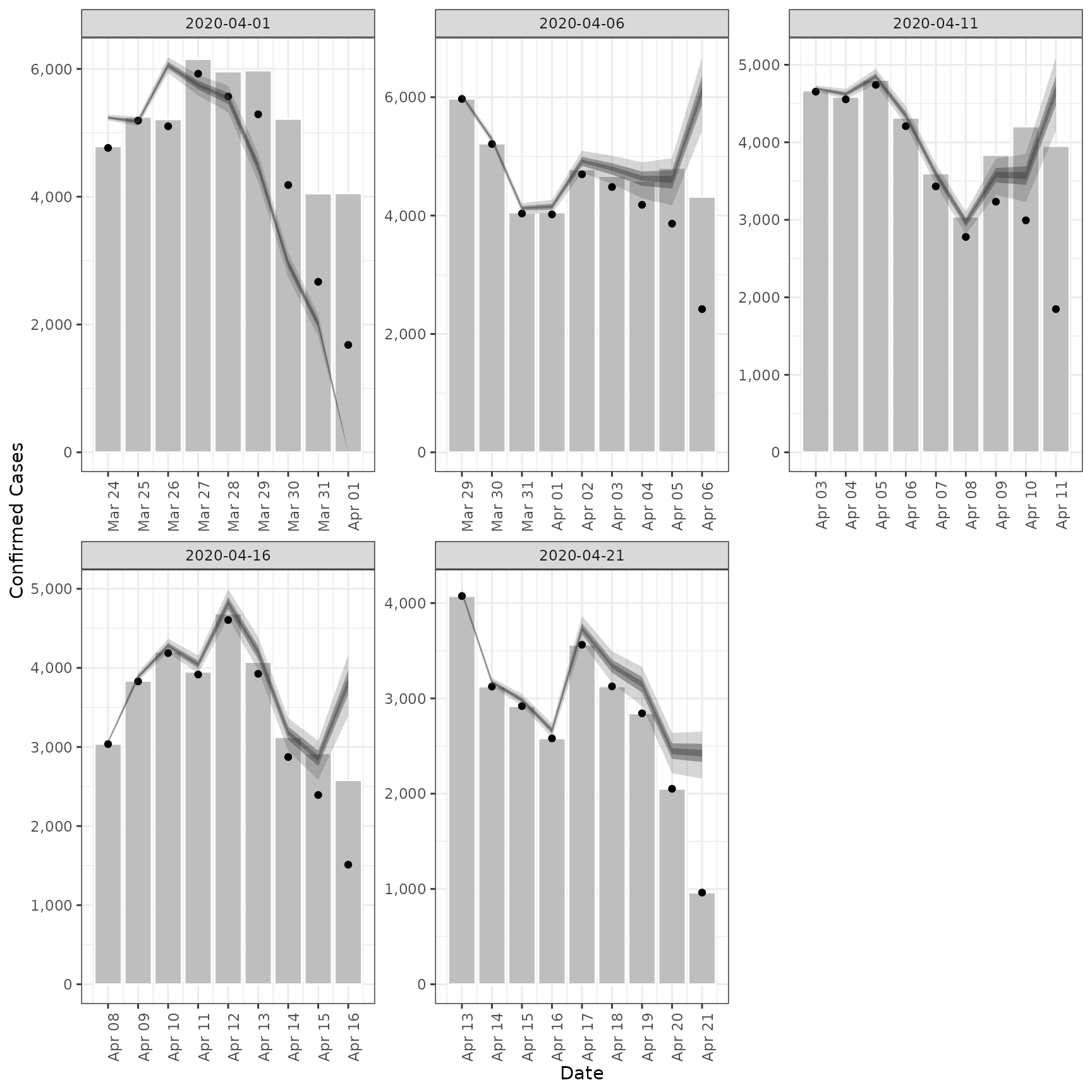
# validation plot of observations vs estimates
plot(est)
#> Ignoring unknown labels:
#> • fill : "Type"


# Pass the truncation distribution to `epinow()`.
# Note, we're using the last snapshot as the observed data as it contains
# all the previous snapshots. Also, we're using the default options for
# illustrative purposes only.
out <- epinow(
  generation_time = generation_time_opts(example_generation_time),
  example_truncated[[5]],
  truncation = trunc_opts(get_parameters(est)[["truncation"]])
)
#> Logging threshold set at INFO for the name logger
#> Writing EpiNow2 logs to the console and:
#> /tmp/Rtmp6mtG43/regional-epinow/2020-04-21.log.
#> Logging threshold set at INFO for the name logger
#> Writing EpiNow2.epinow logs to the console and:
#> /tmp/Rtmp6mtG43/epinow/2020-04-21.log.
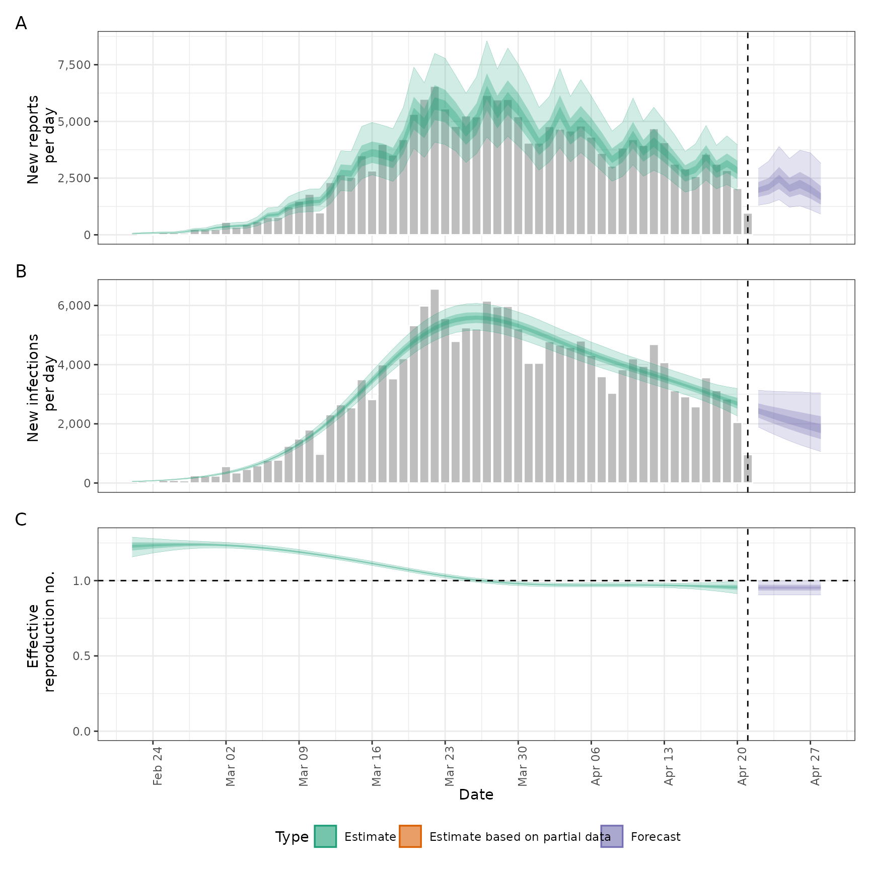
plot(out)

options(old_opts)
# }

Usage

Arguments

Value

See also

Examples