Comparisons

Our estimates and projections set against those other groups have published for the same outbreak.

Load packages, data and fitted chains

# Shared setup: packages, observations and the fit registry. See
# `docs/pages/_setup.jl`.
using BVDOutbreakSize
include(joinpath(pkgdir(BVDOutbreakSize), "docs", "pages", "_setup.jl"))

validation_forecast_from (generic function with 1 method)

# The fits this page reads, loaded from the cache here.
chn_joint = load_fit("joint")
frozen_by_cutoff = frozen_fits_by_cutoff()
frozen_C(c) = vec(Array(frozen_by_cutoff[c].chn[:C_T]))
posterior_C_joint = vec(Array(chn_joint[:C_T]));

Comparison with McCabe et al.

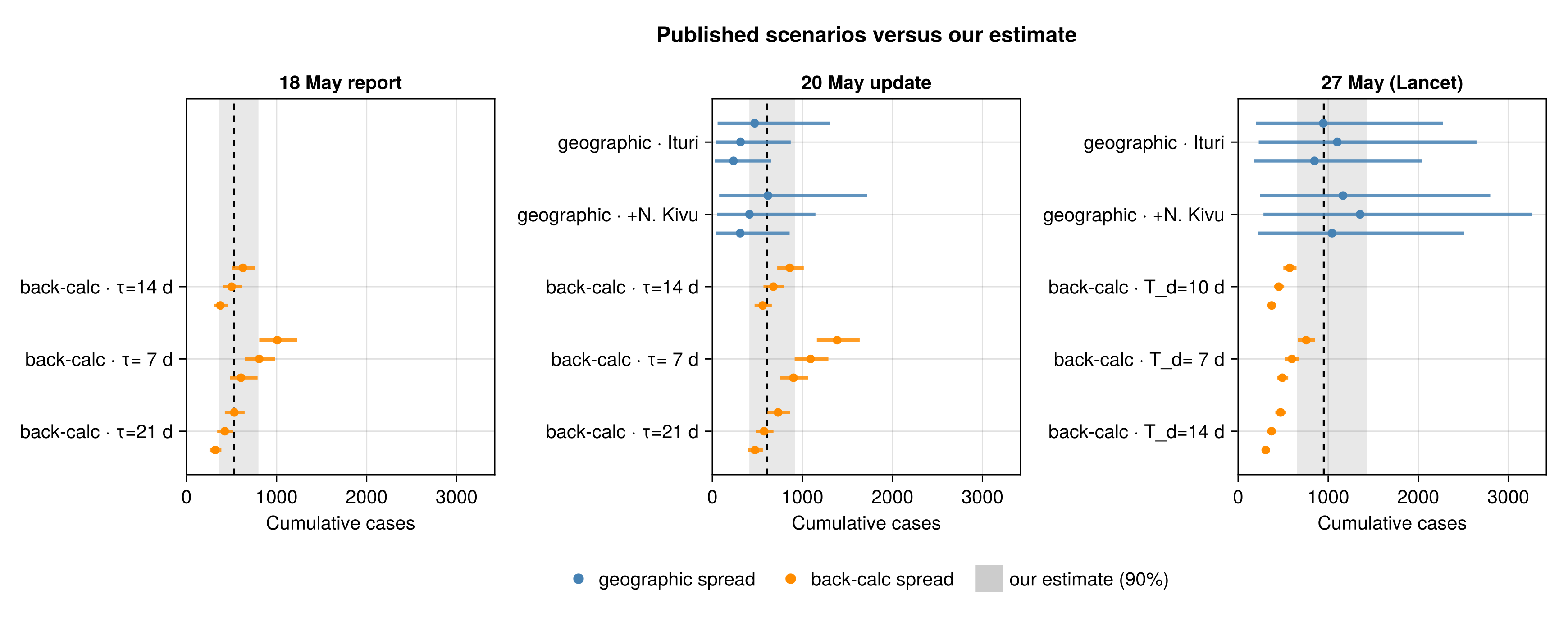
McCabe et al. published their estimates as scenarios at fixed situation-report cut-offs, each scenario carrying a 95% confidence interval. We show all three, the 18 May report, the 20 May update and the 27 May Lancet publication, as one panel each, with their intervals kept. Within a panel each method and scenario family is a single line, carrying its sweep over the nuisance assumptions: the case-fatality ratio, the geographic window and the doubling time. The geographic-spread scenarios come from exported cases and travel volume. Their back-calculation-from-deaths scenarios differ between the reports, since the 18 May report used 88 reported deaths and the 20 May update 131. The 20 May update also corrected the case-fatality ratios. McCabe's scenarios estimate cumulative cases at their report dates, though their report is not fully explicit about whether this is symptomatic cases or all infections. We take the like-for-like quantity to be our cumulative symptom onsets on the same dates, not the latent infections (which include the not-yet-symptomatic) or our current cut-off total. We read our value off the joint fit's cumulative-onset trajectory at the grid day for each report date, and show it with its credible interval.

McCabe scenarios with uncertainty against our estimates

function _ci90row(xs)
    return (
        round(Int, quantile(xs, 0.5)),
        round(Int, quantile(xs, 0.05)),
        round(Int, quantile(xs, 0.95)),
    )
end

# Our modelled cumulative symptom onsets on a McCabe report date, read off
# the joint fit's per-draw `cumulative_onsets` trajectory. The grid runs to
# the cut-off on day `n`, so the day-index for a date is `n` minus the days
# from that date back to the cut-off (`grid_day("2026-06-07") = n`,
# `"2026-05-20") = n - 18`, `"2026-05-18") = n - 20`).
_onset_trajs = let mat = chn_joint[:cumulative_onsets]
    [collect(v) for v in vec(collect(mat))]
end
# Inverse of `grid_date(day) = obs.cutoff - Day(obs.n - day)`: the day-index
# whose calendar date is `date`, using `value` (imported above) for the
# day count rather than the non-exported `Dates.date2epochdays`.
_grid_day(date) = obs.n - value(obs.cutoff - Date(date))
function _ours_on(date)
    d = _grid_day(date)
    return _ci90row(Float64[t[d] for t in _onset_trajs])
end

# Our matched cumulative-onset estimate for each report date, keyed by date so
# it lands beside that vintage's scenarios in its own panel.
mccabe_ours = Dict(
    "2026-05-18" => _ours_on("2026-05-18"),
    "2026-05-20" => _ours_on("2026-05-20"),
    "2026-05-27" => _ours_on("2026-05-27")
)

# One panel per report date; within a panel each method-and-family is one row,
# with the case-fatality / window / doubling-time sweep dodged onto that single
# line, so the ~40 scenarios keep their intervals without becoming ~40 rows.
matched_comparison_fig = plot_scenario_comparison(
    REPORT_SCENARIOS_CI;
    ours = mccabe_ours,
    date_titles = [
        "2026-05-18" => "18 May report",
        "2026-05-20" => "20 May update",
        "2026-05-27" => "27 May (Lancet)",
    ],
    xlabel = "Cumulative cases"
);

Their 95% confidence intervals come from exact negative-binomial counts for the geographic-spread method and a Poisson likelihood profile for the back-calculation from deaths.

Frozen-fit C_T intervals (kept for the CSV export, not shown)

# The frozen-fit infection counts for the published
# `frozen_matched_cutoffs.csv` export, not shown on the page.
frozen_streams_table = streams_table(
    "frozen 20 May" => frozen_C("2026-05-20"),
    "frozen 23 May" => frozen_C("2026-05-23"),
    "frozen 27 May" => frozen_C("2026-05-27"),
    "frozen 8 June" => frozen_C(default_chamla_cutoff()),
    "current data" => posterior_C_joint
);

Comparison with Chamla et al.

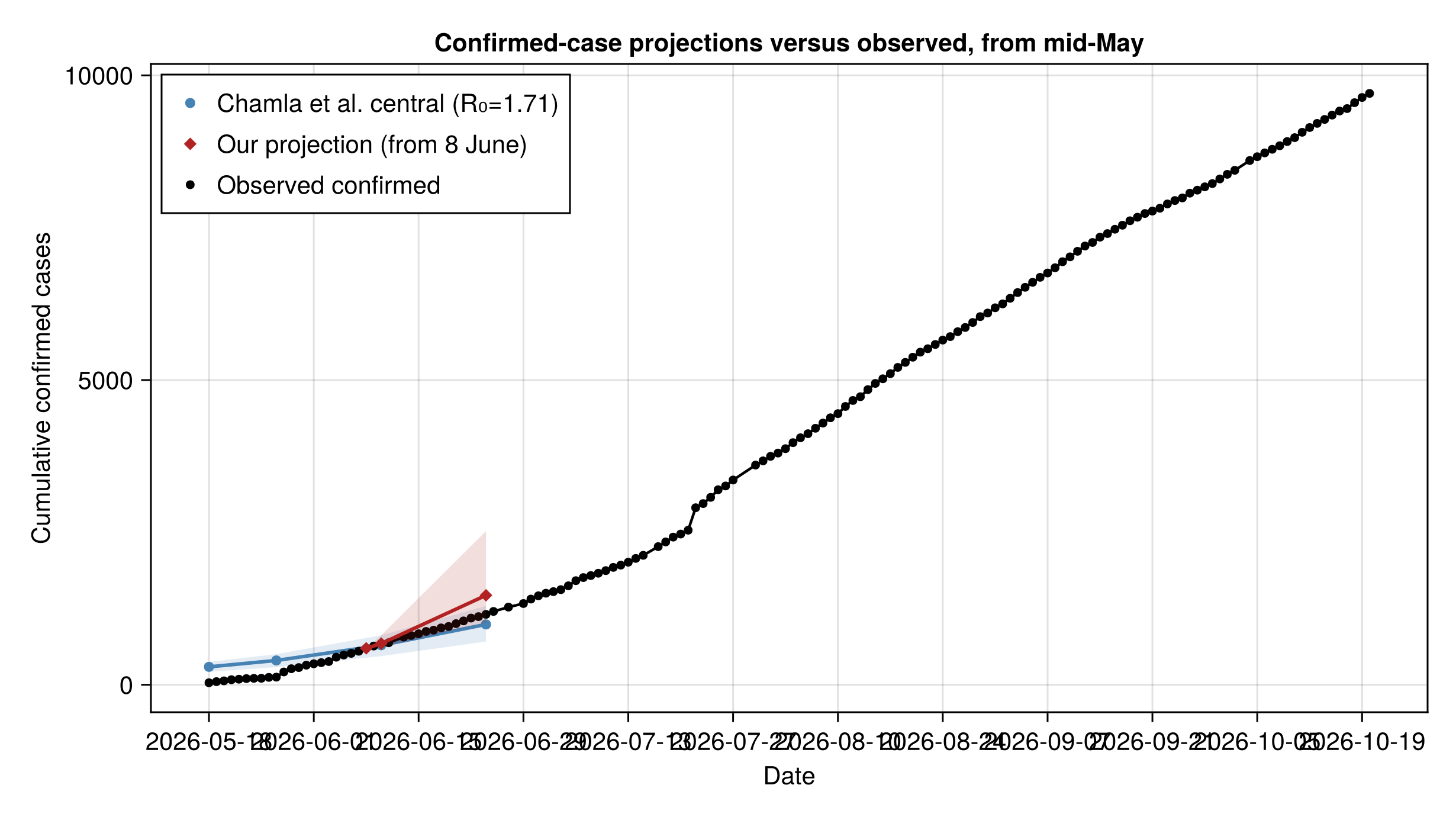
A second group, Chamla et al. (2026) at the World Health Organization Regional Office for Africa, published a stochastic compartmental model of the same outbreak on 25 June 2026. Their model is a discrete-time susceptible-exposed-infectious-recovered-dead ensemble, recalibrated by simulation filtering to the laboratory-confirmed case series and anchored on the 598 confirmed cases reported by 8 June. It is then run forward to project the confirmed-case trajectory under a low, central and high transmissibility scenario.

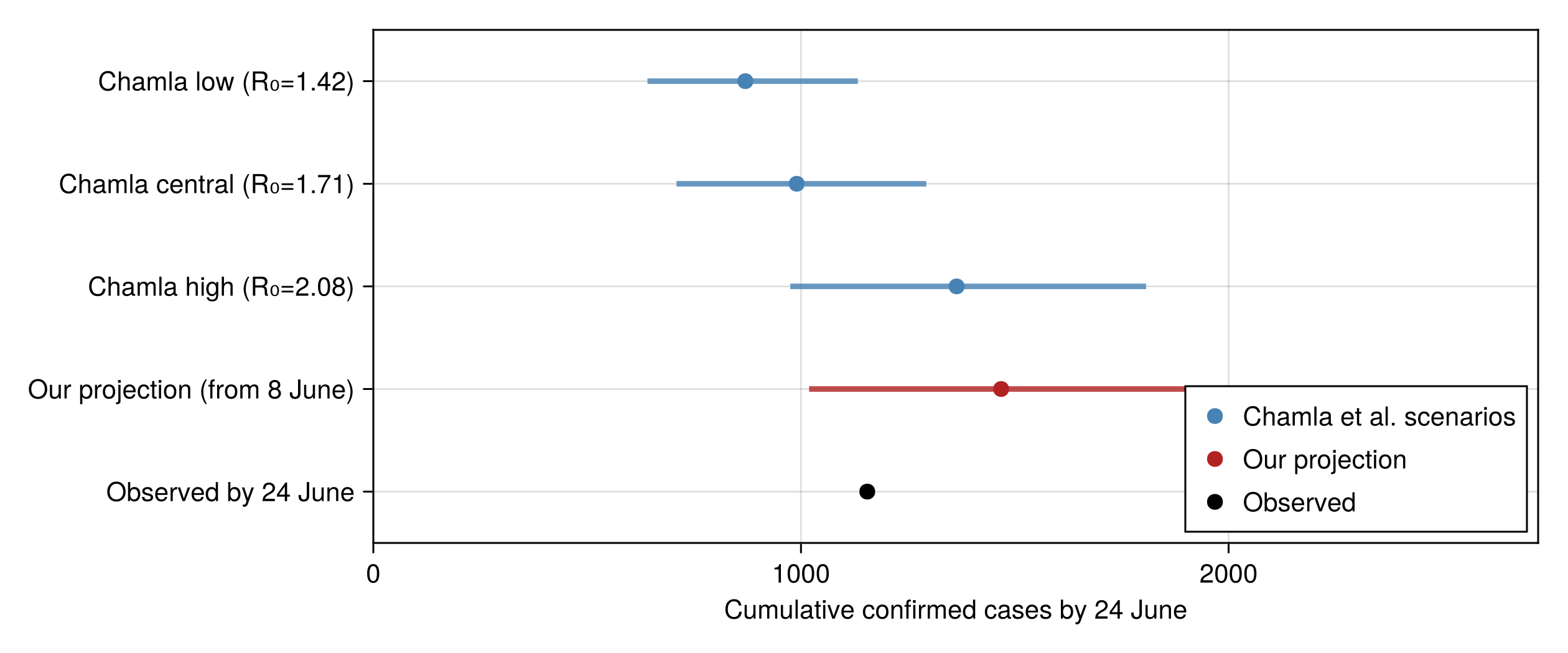
Their published quantity is the cumulative confirmed-case count, with the reporting fraction held at one, so it does not adjust for the cases that are infected but never laboratory-confirmed. This is a different quantity from the cumulative cases this analysis and McCabe et al. estimate, which include the unconfirmed and unascertained. The like-for-like comparison is therefore against our own confirmed-case projection, not against our cumulative infection count.

We compare forward projections rather than refitting to their assumptions. We take our fit frozen at 8 June, the exact date of their confirmed-case calibration anchor. We roll its confirmed-case stream forward to the dates Chamla report, using the same machinery as the one-week-ahead forecast.

Project the 8 June fit forward and assemble the Chamla comparison

# The 8 June frozen joint fit matches Chamla's confirmed-case calibration
# anchor exactly and carries the confirmed-case testing history through then,
# so we forecast its confirmed-case stream to the dates Chamla report.
chamla_anchor = frozen_by_cutoff["2026-06-08"]

# Our projected cumulative confirmed cases at a horizon of `h` days past the
# 8 June cut-off, drawn from the 8 June model run past its cut-off and
# summarised as (median, 5%, 95%).
function _our_confirmed_h(h)
    fc = forecast_reported(
        fit_forecast("frozen_2026-06-08");
        horizon = h,
        obs_cases = chamla_anchor.o.reported_cases,
        obs_deaths = chamla_anchor.o.total_deaths,
        obs_confirmed = chamla_anchor.o.confirmed_cases,
        obs_confirmed_deaths = chamla_anchor.o.confirmed_deaths
    )
    return _ci90row(float.(fc.confirmed_cum))
end

# Our projection at Chamla's forward report dates (10 and 24 June, week 12):
# the anchor day is the fitted confirmed total at 8 June, each later date a
# forward forecast. Reused for the matched-date table and the week-12 figure.
chamla_fan = map(["2026-06-08", "2026-06-10", "2026-06-24"]) do d
    h = value(Date(d) - chamla_anchor.cutoff)
    row = h == 0 ?
        (
            chamla_anchor.o.confirmed_cases, chamla_anchor.o.confirmed_cases,
            chamla_anchor.o.confirmed_cases,
        ) : _our_confirmed_h(h)
    (d, row...)
end
_fan_at(date) =
let r = first(x for x in chamla_fan if x[1] == date)
    (r[2], r[3], r[4])
end
ours_10jun = _fan_at("2026-06-10")
ours_24jun = _fan_at("2026-06-24")

# Observed confirmed totals on Chamla's forward report dates, read from the
# confirmed-case history frozen at each date.
observed_10jun = freeze_observations("2026-06-10").confirmed_cases
observed_24jun = freeze_observations("2026-06-24").confirmed_cases

# Observed confirmed cases over the comparison window: the daily cumulative
# series read off the chain's grid from 18 May (Chamla's first projected point)
# to the cut-off.
chamla_obs_series = let
    ds = [grid_date(d) for d in obs.confirmed_history.days]
    cs = obs.confirmed_history.counts
    [(string(ds[i]), cs[i]) for i in eachindex(ds) if ds[i] >= Date("2026-05-18")]
end

# Chamla's central confirmed-case projection over the comparison window; their
# later, far-larger horizons are noted in the text rather than plotted so the
# window stays legible.
chamla_central_window = CHAMLA_CONFIRMED_CENTRAL[1:4]

chamla_projection_fig = plot_projection_comparison(;
    external = chamla_central_window,
    ours = chamla_fan,
    observed = chamla_obs_series,
    external_label = "Chamla et al. central (R₀=1.71)",
    ours_label = "Our projection (from 8 June)",
    observed_label = "Observed confirmed",
    title = "Confirmed-case projections versus observed, from mid-May"
);

By 24 June their central scenario projected just under a thousand confirmed cases, and their low and high scenarios ranged from roughly 870 to 1360.

Week-12 (24 June) scenario spread against ours and observed

chamla_w12_rows = vcat(
    [(label, m, lo, hi) for (label, m, lo, hi) in CHAMLA_CONFIRMED_W12],
    [("Our projection (from 8 June)", ours_24jun...)],
    [
        (
            "Observed by 24 June", observed_24jun,
            observed_24jun, observed_24jun,
        ),
    ]
)
chamla_w12_groups = vcat(
    fill("Chamla et al. scenarios", 3),
    ["Our projection"], ["Observed"]
)

chamla_w12_fig = plot_estimate_comparison(
    chamla_w12_rows;
    xlabel = "Cumulative confirmed cases by 24 June",
    groups = chamla_w12_groups,
    group_colours = [
        "Chamla et al. scenarios" => :steelblue,
        "Our projection" => :firebrick,
        "Observed" => :black,
    ]
);

Matched-date projection numbers (10 and 24 June)

chamla_comparison_table = let
    fmt(t) = string(t[1], " (", t[2], "–", t[3], ")")
    central(date) =
    let r = first(
            x for x in CHAMLA_CONFIRMED_CENTRAL
                if x[1] == date
        )
        fmt((r[2], r[3], r[4]))
    end
    DataFrame(
        "Date" => ["10 June", "24 June"],
        "Chamla central (90% PI)" => [
            central("2026-06-10"),
            central("2026-06-24"),
        ],
        "Our projection (90% CrI)" => [fmt(ours_10jun), fmt(ours_24jun)],
        "Observed confirmed" => [
            string(observed_10jun),
            string(observed_24jun),
        ]
    )
end;

Date	Chamla central (90% PI)	Our projection (90% CrI)	Observed confirmed
10 June	648 (470–812)	674 (618–799)	676
24 June	990 (709–1293)	1452 (1007–2420)	1155

Beyond the comparison window their central scenario continues to roughly 8200 confirmed cases by mid-September, with the high scenario far higher.

Reproduction number behind the projection

The forward projection above is carried by the reproduction-number trajectory our 8 June fit estimated, a quantity we report in its own right rather than as a comparison. It declines over the weeks leading to the cut-off, and that decline is what bends the projected trajectory away from sustained early growth.

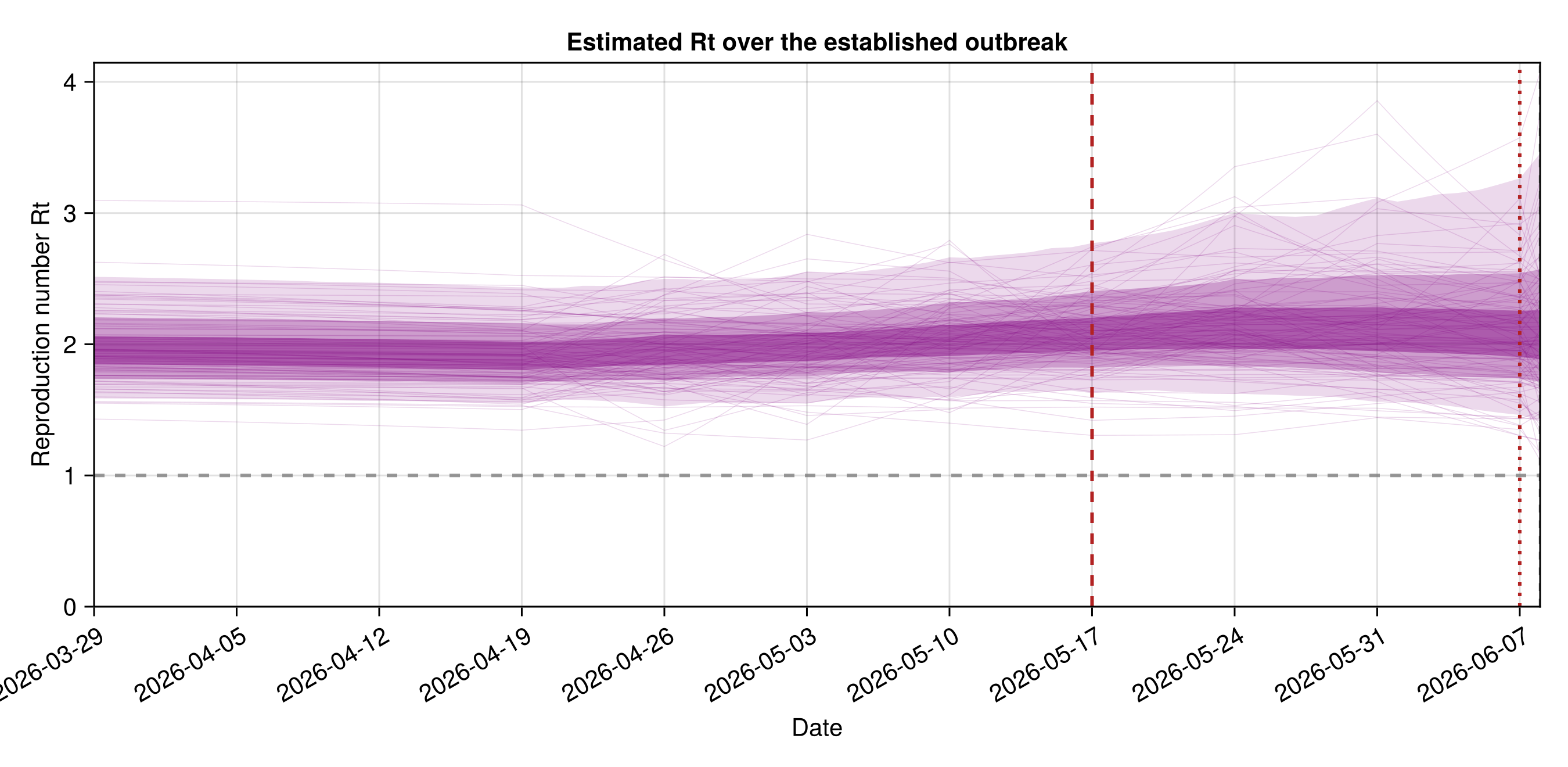
Reproduction number as estimated by the 8 June fit

# Reconstruct the reproduction-number trajectory the 8 June fit estimated,
# mirroring the current-data R_t figure but with the frozen vintage's own grid,
# breakpoint and renewal start.
chamla_rt_obs = chamla_anchor.o
chamla_rt_breakpoint = chamla_rt_obs.n - chamla_rt_obs.who_first_sitrep_days
chamla_rt_start = clamp(
    chamla_rt_obs.n - round(Int, chamla_rt_obs.tmrca_days) + RENEWAL_START_LEAD,
    1, chamla_rt_obs.n
)
chamla_rt_fig = plot_rt(
    chamla_anchor.chn;
    n = chamla_rt_obs.n, breakpoint = chamla_rt_breakpoint,
    rt_start = chamla_rt_start,
    rt_walk_start = clamp(
        chamla_rt_breakpoint - RT_WALK_LEAD,
        chamla_rt_start, chamla_rt_obs.n
    ),
    as_of_date = string(chamla_rt_obs.cutoff),
    seeding = chamla_rt_obs.seeding, ramp = RT_INTERVENTION_RAMP
);

Saving comparison outputs

The frozen-fit table is written to the shared output directory.

Write comparison outputs

output_dir = get(
    ENV, "BVD_OUTPUT_DIR",
    joinpath(pkgdir(BVDOutbreakSize), "output")
)
mkpath(output_dir)
CSV.write(
    joinpath(output_dir, "frozen_matched_cutoffs.csv"),
    frozen_streams_table
)

"/home/runner/work/BVDOutbreakSize/BVDOutbreakSize/output/frozen_matched_cutoffs.csv"