Health-zone in-sample checks
This page checks whether the health-zone model reproduces the per-zone data it was fitted to. The national checks are on the national in-sample checks page and the provincial ones on the province in-sample checks page. The zone data enter the model as compositions of their patch's totals, so the checks are on each zone's share of its patch. A later section sets each zone's reproduction number from the current fit against the same fit a week earlier, and the last follows each zone's published estimates across releases.
Load packages, data and fitted chains
# Shared setup: packages, observations and the fit registry. See
# `docs/pages/_setup.jl`.
using BVDOutbreakSize
include(joinpath(pkgdir(BVDOutbreakSize), "docs", "pages", "_setup.jl"))
validation_forecast_from (generic function with 1 method)# The fits this page reads, loaded from the cache here. The headline joint
# carries the patch trajectories the zone stage conditions on, and the
# frozen zone fit is the same fit a week earlier.
chn_joint = load_fit("joint");
chn_local = load_fit("local");
frozen_local = load_fit("local_frozen_validation");Summary
The overall bullets come first, then a table of each province's bias and coverage, from the zone composition calibration below. A cell is one zone at one vintage, and a composition that was not scored reads n/a. Bias and coverage are defined as on the national in-sample checks page, with a nominal coverage of 0.9.
Least well reproduced: Haut-Uele (cases), Tshopo (cases) and Bas-Uele (cases) have the largest absolute bias.
Coverage: 16 of 16 composition rows have 90% coverage of at least 0.8; the lowest is Haut-Uele (cases) at 0.96.
Province levels: over the last two weeks the zone stage's infections are within 36.8% of the joint model's in every province, the furthest being Sud-Ubangi.
| Province | Stream | Bias | 90% coverage | Cells |
|---|---|---|---|---|
| Ituri | Confirmed cases | 0 | 0.97 | 4060 |
| Ituri | Confirmed deaths | 0 | 0.98 | 3976 |
| Nord-Kivu | Confirmed cases | 0 | 0.98 | 2380 |
| Nord-Kivu | Confirmed deaths | 0 | 0.98 | 2278 |
| Haut-Uele | Confirmed cases | 0.03 | 0.96 | 832 |
| Haut-Uele | Confirmed deaths | 0.01 | 0.98 | 704 |
| Sud-Kivu | Confirmed cases | 0 | 1 | 1 |
| Sud-Kivu | Confirmed deaths | 0 | 1 | 1 |
| Tshopo | Confirmed cases | 0.02 | 0.97 | 364 |
| Tshopo | Confirmed deaths | 0 | 0.99 | 203 |
| Bas-Uele | Confirmed cases | 0.01 | 1 | 30 |
| Bas-Uele | Confirmed deaths | 0 | 1 | 12 |
| Sud-Ubangi | Confirmed cases | 0 | 1 | 2 |
| Sud-Ubangi | Confirmed deaths | 0 | 1 | 1 |
| Nord-Ubangi | Confirmed cases | 0 | 1 | 12 |
| Nord-Ubangi | Confirmed deaths | 0 | 1 | 2 |
Zone compositions
The zone compositions sit one level below the province compositions. Cases and deaths are separate compositions in the zone observations, so the two are checked separately.
Load the zone fit's inputs and prior
# `zone_stage_inputs` and `zone_prior_draws` are defined in the shared setup,
# so the zone estimates and forecast pages read the same fixed inputs.
zone_inputs = zone_stage_inputs();
zone_patch = zone_inputs.patch_of_zone;
prior_chn_zone = zone_prior_draws(zone_inputs);
Confirmed cases
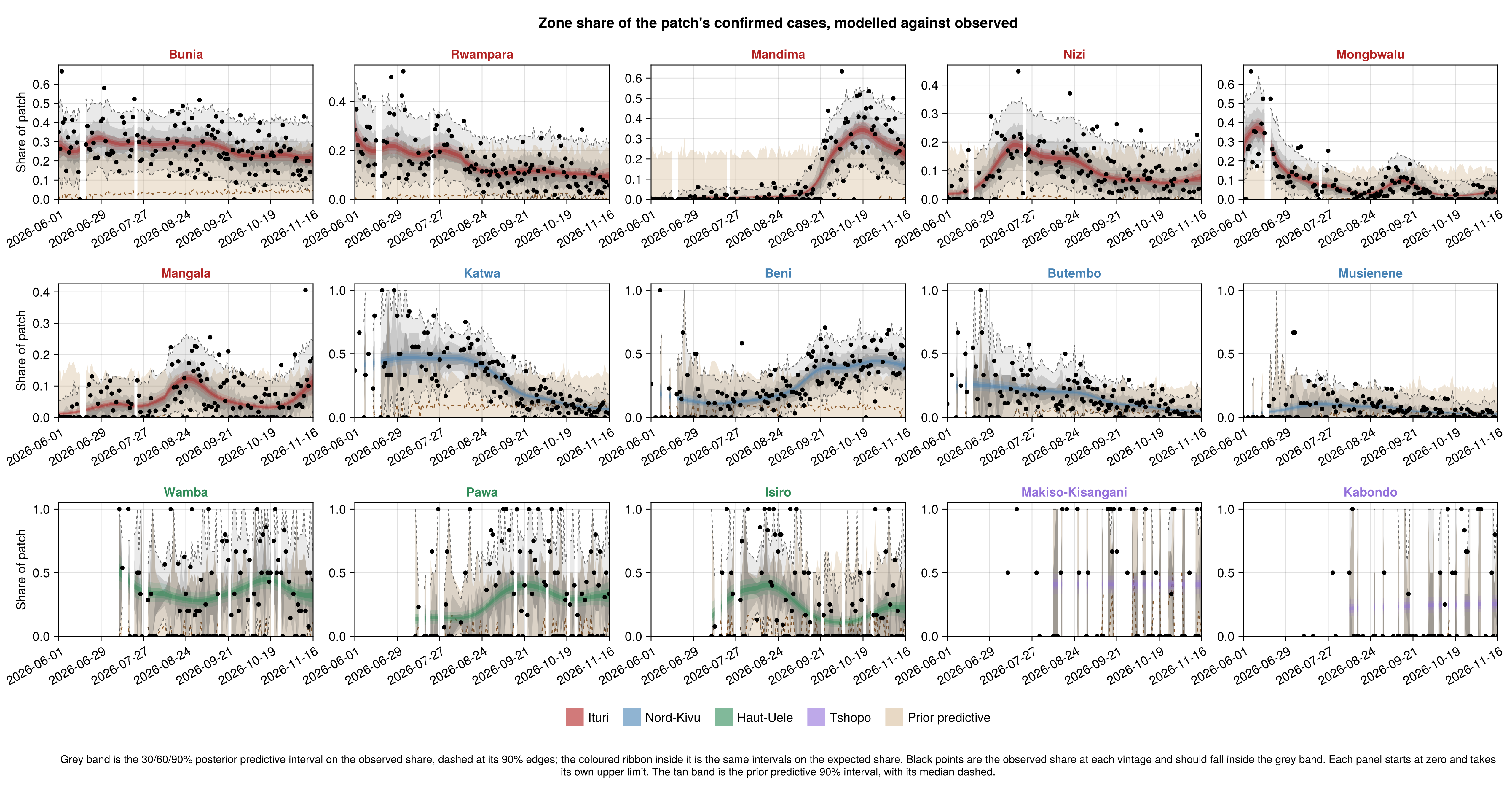
Zone case composition predictive checks
# Per-draw expected, predictive and observed zone shares at every vintage,
# from the posterior and from the zone prior, per vintage and cumulative.
zone_ppc = zone_composition_draws(chn_local, zone_inputs);
zone_ppc_prior = zone_composition_draws(prior_chn_zone, zone_inputs);
zone_ppc_cum = zone_composition_draws(
    chn_local, zone_inputs;
    cumulative = true
);
zone_ppc_prior_cum = zone_composition_draws(
    prior_chn_zone, zone_inputs;
    cumulative = true
);
zone_ppc_fig = plot_zone_shares(
    zone_ppc.expected, zone_ppc.observed,
    zone_inputs.dates, zone_inputs.zone_labels;
    zone_patch, patch_labels = zone_inputs.patch_labels,
    pred_draws = zone_ppc.predictive_share,
    prior_draws = zone_ppc_prior.predictive_share, top = 15, ncols = 5
);
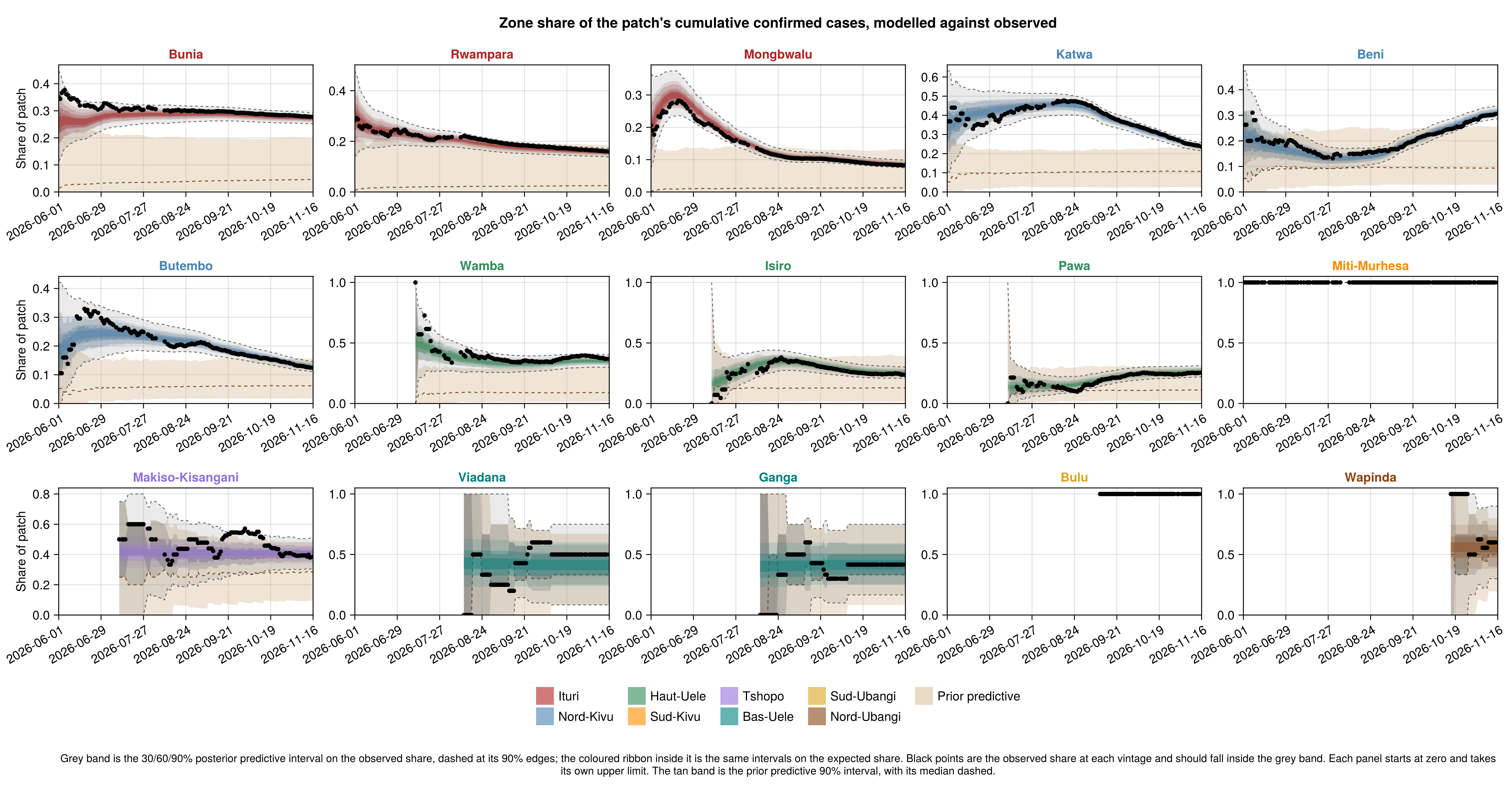
zone_ppc_cum_fig = plot_zone_shares(
    zone_ppc_cum.expected,
    zone_ppc_cum.observed, zone_inputs.dates, zone_inputs.zone_labels;
    zone_patch, patch_labels = zone_inputs.patch_labels,
    pred_draws = zone_ppc_cum.predictive_share,
    prior_draws = zone_ppc_prior_cum.predictive_share, top = 15, ncols = 5,
    title = "Zone share of the patch's cumulative confirmed cases, " *
        "modelled against observed"
);
Confirmed deaths
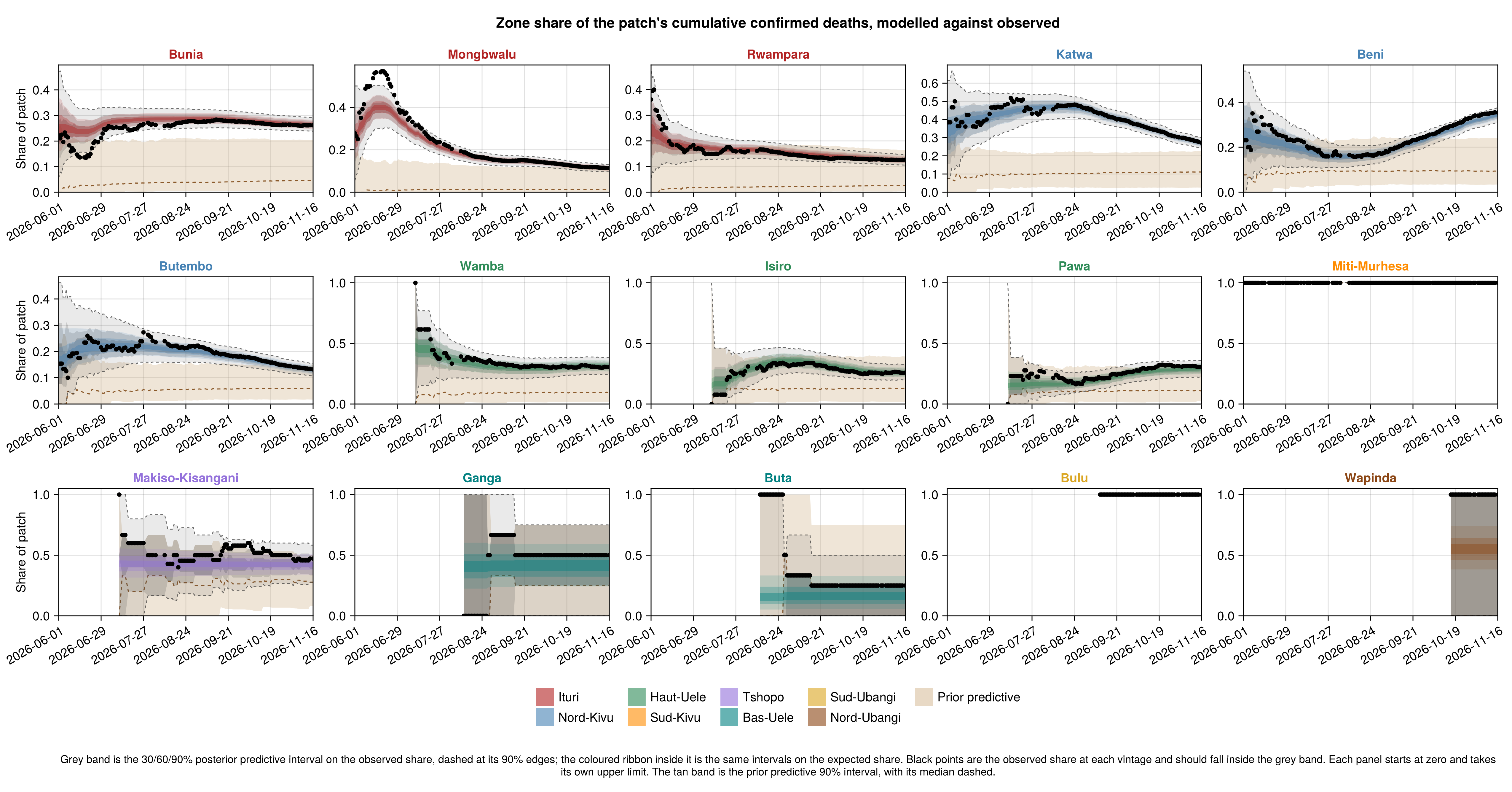
Zone death composition predictive check
zone_death_ppc_cum = zone_composition_draws(
    chn_local, zone_inputs;
    stream = :deaths, cumulative = true
);
zone_death_ppc_prior_cum = zone_composition_draws(
    prior_chn_zone, zone_inputs;
    stream = :deaths, cumulative = true
);
zone_death_ppc_cum_fig = plot_zone_shares(
    zone_death_ppc_cum.expected, zone_death_ppc_cum.observed,
    zone_inputs.dates, zone_inputs.zone_labels;
    zone_patch, patch_labels = zone_inputs.patch_labels,
    pred_draws = zone_death_ppc_cum.predictive_share,
    prior_draws = zone_death_ppc_prior_cum.predictive_share,
    top = 15, ncols = 5,
    title = "Zone share of the patch's cumulative confirmed deaths, " *
        "modelled against observed"
);
Zone composition calibration
Both compositions are scored the way the stream calibration scores the national streams, over every zone and vintage of each patch.
Zone composition calibration
# The two compositions in one table, each patch row named by the
# composition it belongs to so the calibration plot reads them apart.
zone_calibration_table = let
    function tagged(stream, what)
        tbl = zone_composition_calibration(
            chn_local, zone_inputs; stream = stream
        )
        tbl[!, "Stream"] = string.(tbl[!, "Stream"], " ($what)")
        return tbl
    end
    vcat(tagged(:cases, "cases"), tagged(:deaths, "deaths"))
end;
zone_calibration_fig = plot_stream_calibration(zone_calibration_table);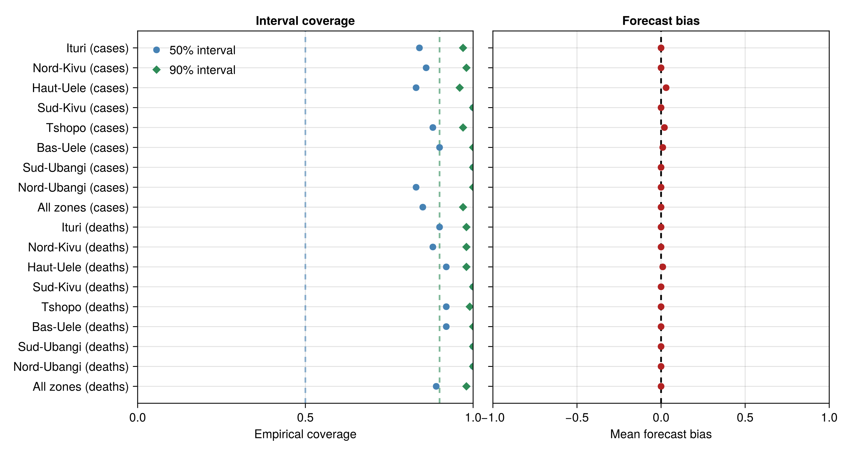
| Stream | Vintages | Bias | 50% coverage | 90% coverage |
|---|---|---|---|---|
| Ituri (cases) | 4060 | 0 | 0.84 | 0.97 |
| Nord-Kivu (cases) | 2380 | 0 | 0.86 | 0.98 |
| Haut-Uele (cases) | 832 | 0.03 | 0.83 | 0.96 |
| Sud-Kivu (cases) | 1 | 0 | 1 | 1 |
| Tshopo (cases) | 364 | 0.02 | 0.88 | 0.97 |
| Bas-Uele (cases) | 30 | 0.01 | 0.9 | 1 |
| Sud-Ubangi (cases) | 2 | 0 | 1 | 1 |
| Nord-Ubangi (cases) | 12 | 0 | 0.83 | 1 |
| All zones (cases) | 7681 | 0 | 0.85 | 0.97 |
| Ituri (deaths) | 3976 | 0 | 0.9 | 0.98 |
| Nord-Kivu (deaths) | 2278 | 0 | 0.88 | 0.98 |
| Haut-Uele (deaths) | 704 | 0.01 | 0.92 | 0.98 |
| Sud-Kivu (deaths) | 1 | 0 | 1 | 1 |
| Tshopo (deaths) | 203 | 0 | 0.92 | 0.99 |
| Bas-Uele (deaths) | 12 | 0 | 0.92 | 1 |
| Sud-Ubangi (deaths) | 1 | 0 | 1 | 1 |
| Nord-Ubangi (deaths) | 2 | 0 | 1 | 1 |
| All zones (deaths) | 7177 | 0 | 0.89 | 0.98 |
Province levels
The zone model scores compositions within each province, so it should produce province infection estimates equivalent to the joint model. The table sets the zone infections summed over each province against the joint model's infections there, as the posterior mean over each of the last four weeks to the cut-off.
Zone stage against joint infections by province
# The zone stage's patch infections against the joint's draws they were
# melded from, per week and province.
zone_level_table = let tbl = zone_patch_level_check(
        chn_local, zone_inputs, chn_joint
    )
    tbl[!, "Zone stage"] = round.(tbl[!, "Zone stage"]; digits = 0)
    tbl[!, "Joint"] = round.(tbl[!, "Joint"]; digits = 0)
    tbl[!, "Ratio"] = round.(tbl[!, "Ratio"]; digits = 3)
    tbl
end;| Province | Week ending | Zone stage | Joint | Ratio |
|---|---|---|---|---|
| Ituri | 2026-10-26 | 432 | 432 | 0.999 |
| Nord-Kivu | 2026-10-26 | 397 | 399 | 0.994 |
| Haut-Uele | 2026-10-26 | 61 | 60 | 1.006 |
| Sud-Kivu | 2026-10-26 | 0 | 0 | 0.758 |
| Tshopo | 2026-10-26 | 15 | 15 | 0.987 |
| Bas-Uele | 2026-10-26 | 1 | 1 | 0.947 |
| Sud-Ubangi | 2026-10-26 | 0 | 0 | 0.725 |
| Nord-Ubangi | 2026-10-26 | 3 | 3 | 1.013 |
| All provinces | 2026-10-26 | 908 | 911 | 0.997 |
| Ituri | 2026-11-02 | 422 | 422 | 1 |
| Nord-Kivu | 2026-11-02 | 390 | 393 | 0.992 |
| Haut-Uele | 2026-11-02 | 67 | 67 | 0.997 |
| Sud-Kivu | 2026-11-02 | 0 | 0 | 0.742 |
| Tshopo | 2026-11-02 | 15 | 15 | 0.983 |
| Bas-Uele | 2026-11-02 | 1 | 1 | 0.914 |
| Sud-Ubangi | 2026-11-02 | 0 | 0 | 0.699 |
| Nord-Ubangi | 2026-11-02 | 3 | 3 | 1.023 |
| All provinces | 2026-11-02 | 899 | 902 | 0.996 |
| Ituri | 2026-11-09 | 416 | 415 | 1.004 |
| Nord-Kivu | 2026-11-09 | 392 | 396 | 0.988 |
| Haut-Uele | 2026-11-09 | 74 | 74 | 0.996 |
| Sud-Kivu | 2026-11-09 | 0 | 0 | 0.719 |
| Tshopo | 2026-11-09 | 16 | 16 | 0.98 |
| Bas-Uele | 2026-11-09 | 1 | 1 | 0.871 |
| Sud-Ubangi | 2026-11-09 | 0 | 0 | 0.669 |
| Nord-Ubangi | 2026-11-09 | 4 | 4 | 1.031 |
| All provinces | 2026-11-09 | 903 | 907 | 0.996 |
| Ituri | 2026-11-16 | 414 | 415 | 0.998 |
| Nord-Kivu | 2026-11-16 | 397 | 407 | 0.977 |
| Haut-Uele | 2026-11-16 | 82 | 84 | 0.982 |
| Sud-Kivu | 2026-11-16 | 0 | 0 | 0.687 |
| Tshopo | 2026-11-16 | 16 | 17 | 0.968 |
| Bas-Uele | 2026-11-16 | 1 | 1 | 0.818 |
| Sud-Ubangi | 2026-11-16 | 0 | 0 | 0.632 |
| Nord-Ubangi | 2026-11-16 | 5 | 5 | 1.005 |
| All provinces | 2026-11-16 | 915 | 928 | 0.986 |
Change over the past week
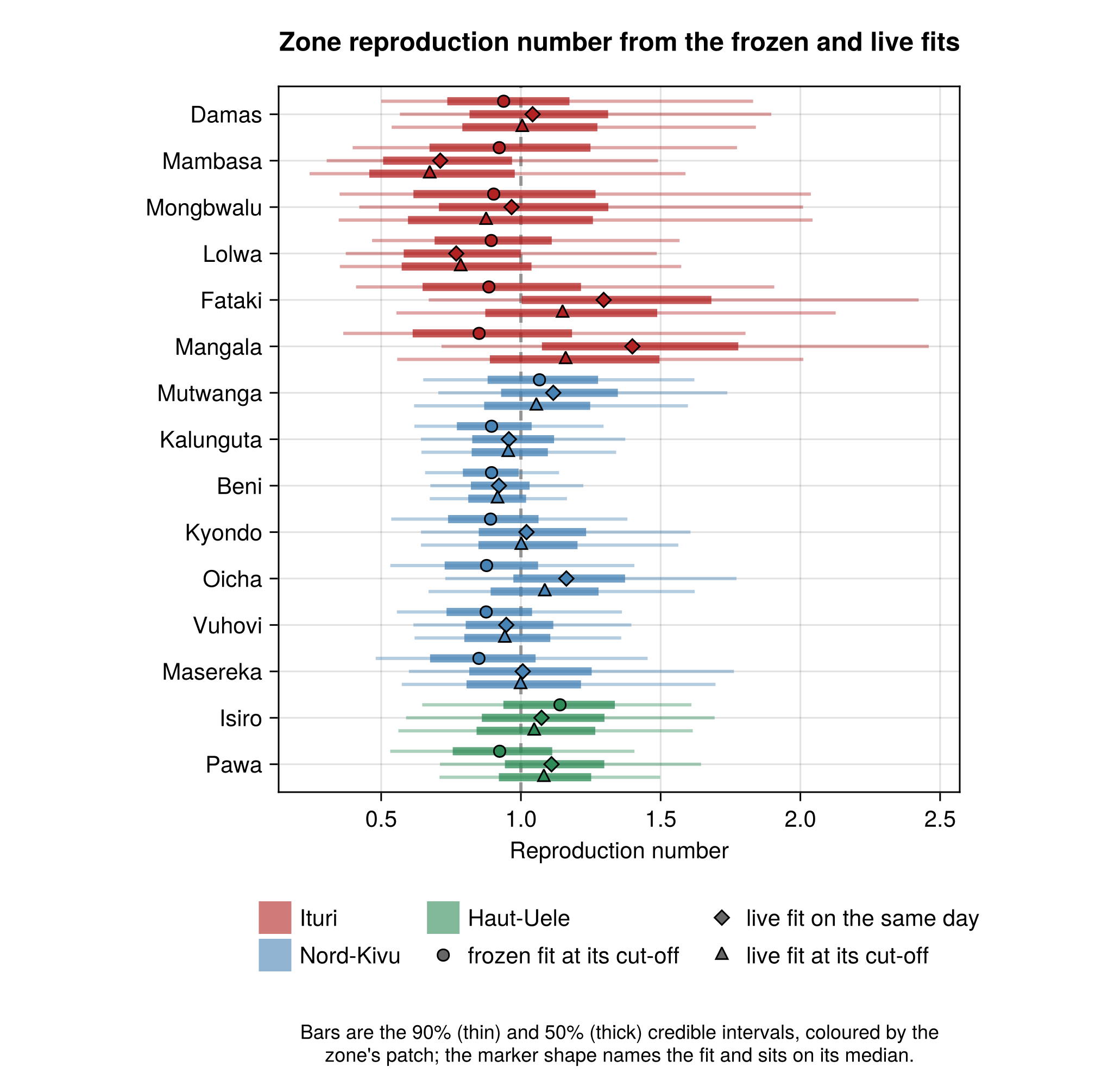
The comparison reads each zone's reproduction number on the frozen cut-off day from the frozen and live fits, alongside the live estimate at the current cut-off. The two fits condition on different weeks of data and on different parent fits. A zone carries its own walk only once it has reported 30 confirmed cases, so the comparison is restricted to zones walking in both fits.
Zone cut-off summaries shared by the comparisons
# The frozen fit's fixed inputs, from the shared setup.
frozen_zone_inputs = frozen_zone_stage_inputs();

# One row per zone in `zs` with the median and the 50% and 90% intervals
# of its draws (one vector per zone), in the schema the zone dot plots
# read, plus the zone's key to match variants by and its confirmed cases
# to rank by. A zone with no finite draw is left out.
function _zone_cutoff_summary(draws, inputs, zs = eachindex(draws))
    keep = [i for (i, v) in enumerate(draws) if any(isfinite, v)]
    z = zs[keep]
    tbl = zone_summary_table(
        [filter(isfinite, draws[i]) for i in keep],
        inputs.zone_labels[z], inputs.patch_of_zone[z]
    )
    tbl.key = inputs.zone_keys[z]
    tbl.cases = inputs.cumulative[z]
    return tbl
end

# The `top` zones by confirmed cases in the first variant, one column per
# variant for the reproduction number. Each cell is a median with its 90%
# interval. Variants are matched by zone key.
function _zone_comparison_table(variants; top::Integer = 10)
    function cell(t, key, d, scale)
        i = findfirst(==(key), t.key)
        i === nothing && return ""
        f(x) = string(round(scale * x; digits = d))
        return string(f(t.median[i]), " (", f(t.lo90[i]), "–", f(t.hi90[i]), ")")
    end
    base = first(last(first(variants)))
    order = sortperm(base.cases; rev = true)[1:min(top, size(base, 1))]
    df = DataFrame(
        "Zone" => base.label[order],
        "Province" => [PROVINCE_LABELS[p] for p in base.patch[order]],
        "Cases" => base.cases[order]
    )
    for (q, name, d, scale) in ((:R, "R", 2, 1),),
            (label, s) in variants

        haskey(s, q) || continue
        df[!, "$name ($label)"] = [
            cell(s[q], k, d, scale)
                for k in base.key[order]
        ]
    end
    return df
end
_zone_comparison_table (generic function with 1 method)Zone reproduction numbers from the frozen and live fits
# Daily reproduction numbers rebuilt from both fits, and the zones walking
# in both as live index => frozen index, matched by key. The summaries
# take their labels and cases from the live inputs.
zone_rt_live = reconstruct_zone_rt(chn_local, zone_inputs)
zone_rt_frozen = reconstruct_zone_rt(frozen_local.chn, frozen_zone_inputs)
zone_week_pairs = [
    z => j
        for (z, k) in enumerate(zone_inputs.zone_keys)
        for j in (findfirst(==(k), frozen_zone_inputs.zone_keys),)
        if j !== nothing && zone_inputs.walking[z] &&
        frozen_zone_inputs.walking[j]
]
zone_week_variants = let zs = first.(zone_week_pairs), js = last.(zone_week_pairs),
        n_f = frozen_zone_inputs.n

    [
        "frozen fit at its cut-off" => (;
            R = _zone_cutoff_summary(
                [zone_rt_frozen[j][:, n_f] for j in js],
                zone_inputs, zs
            ),
        ),
        "live fit on the same day" => (;
            R = _zone_cutoff_summary(
                [zone_rt_live[z][:, n_f] for z in zs],
                zone_inputs, zs
            ),
        ),
        "live fit at its cut-off" => (;
            R = _zone_cutoff_summary(
                [zone_rt_live[z][:, end] for z in zs],
                zone_inputs, zs
            ),
        ),
    ]
end
zone_week_table = _zone_comparison_table(zone_week_variants);
zone_week_fig = plot_zone_comparison(
    [l => s.R for (l, s) in zone_week_variants];
    xlabel = "Reproduction number", reference_line = 1.0,
    title = "Zone reproduction number from the frozen and live fits"
);

# The frozen trajectories padded onto the live grid, undefined past the
# frozen cut-off, behind the live ones over the zone grid. The plot reads
# an undefined day as `missing`, where the reconstruction writes `NaN`.
zone_week_rt_fig = let grid = zone_inputs.t0:obs.n, n_f = frozen_zone_inputs.n
    asmissing(m) = replace(m, NaN => missing)
    frozen = map(zone_week_pairs) do (z, j)
        m = fill(NaN, size(zone_rt_frozen[j], 1), obs.n)
        m[:, 1:n_f] .= zone_rt_frozen[j]
        asmissing(m[:, grid])
    end
    zs = first.(zone_week_pairs)
    plot_rt_zones(
        [asmissing(zone_rt_live[z][:, grid]) for z in zs],
        zone_inputs.zone_labels[zs], zone_inputs.patch_of_zone[zs];
        patch_labels = zone_inputs.patch_labels,
        dates = grid_date.(grid), as_of_date = obs.cutoff,
        ranking = zone_inputs.cumulative[zs],
        ranking_label = "confirmed cases to date", top = 12,
        reference_rt = frozen, reference_label = "Frozen fit",
        title = "Zone reproduction number from the live fit, " *
            "with the frozen fit behind"
    )
end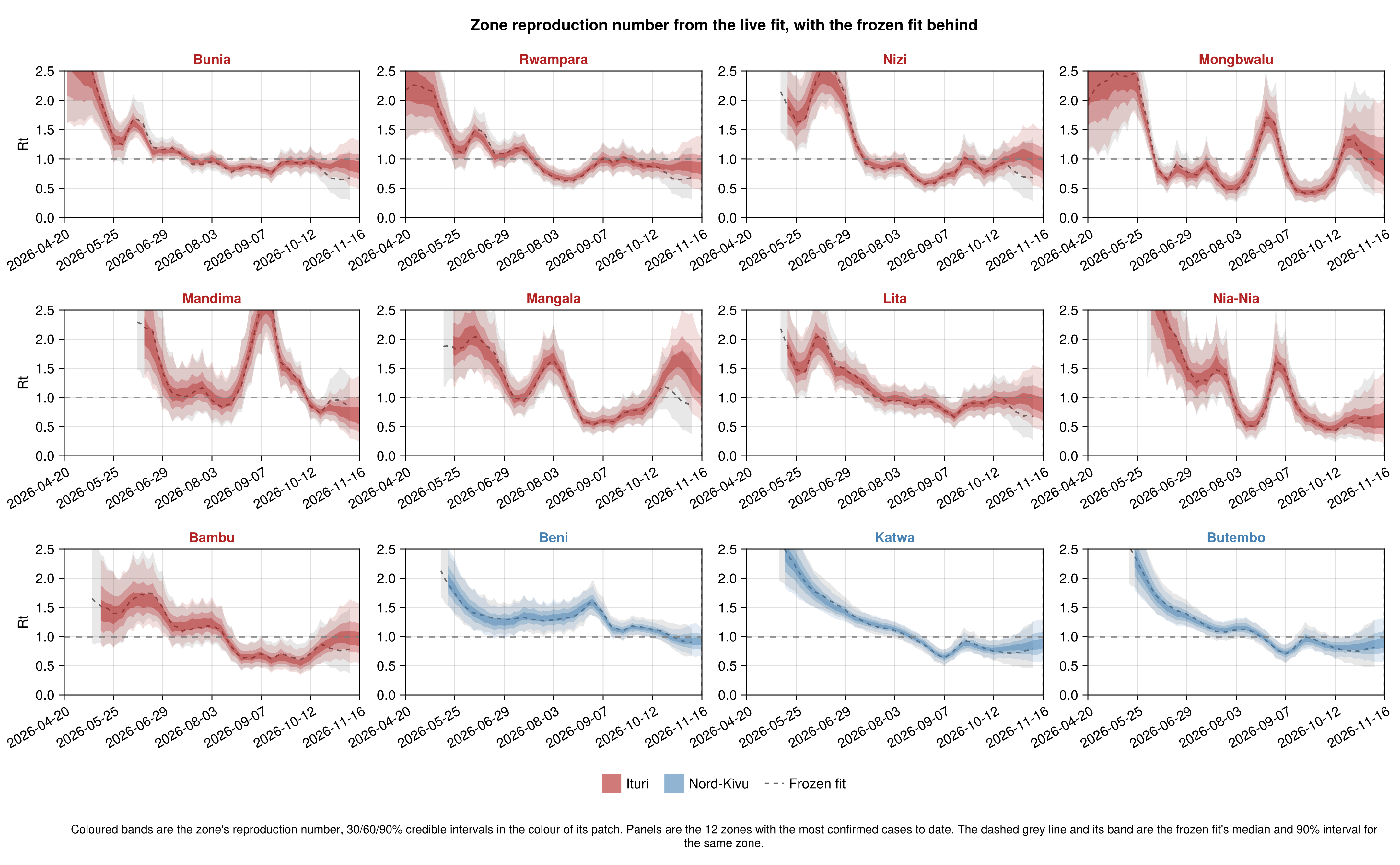
| Zone | Province | Cases | R (frozen fit at its cut-off) | R (live fit on the same day) | R (live fit at its cut-off) |
|---|---|---|---|---|---|
| Bunia | Ituri | 2105 | 0.67 (0.31–1.15) | 0.89 (0.53–1.35) | 0.85 (0.48–1.32) |
| Rwampara | Ituri | 1235 | 0.68 (0.31–1.22) | 0.86 (0.5–1.36) | 0.84 (0.45–1.41) |
| Beni | Nord-Kivu | 905 | 0.89 (0.66–1.14) | 0.92 (0.68–1.22) | 0.92 (0.67–1.16) |
| Nizi | Ituri | 883 | 0.68 (0.27–1.39) | 0.98 (0.54–1.61) | 0.9 (0.47–1.52) |
| Mongbwalu | Ituri | 740 | 0.9 (0.35–2.04) | 0.97 (0.42–2.01) | 0.88 (0.35–2.04) |
| Katwa | Nord-Kivu | 698 | 0.8 (0.46–1.26) | 0.85 (0.56–1.26) | 0.88 (0.57–1.31) |
| Mandima | Ituri | 639 | 0.83 (0.36–1.38) | 0.71 (0.3–1.35) | 0.67 (0.23–1.38) |
| Mangala | Ituri | 460 | 0.85 (0.36–1.8) | 1.4 (0.72–2.46) | 1.16 (0.56–2.01) |
| Butembo | Nord-Kivu | 356 | 0.82 (0.48–1.29) | 0.86 (0.56–1.28) | 0.89 (0.57–1.33) |
| Lita | Ituri | 352 | 0.68 (0.27–1.4) | 0.91 (0.48–1.56) | 0.85 (0.42–1.51) |
Estimate evolution across releases
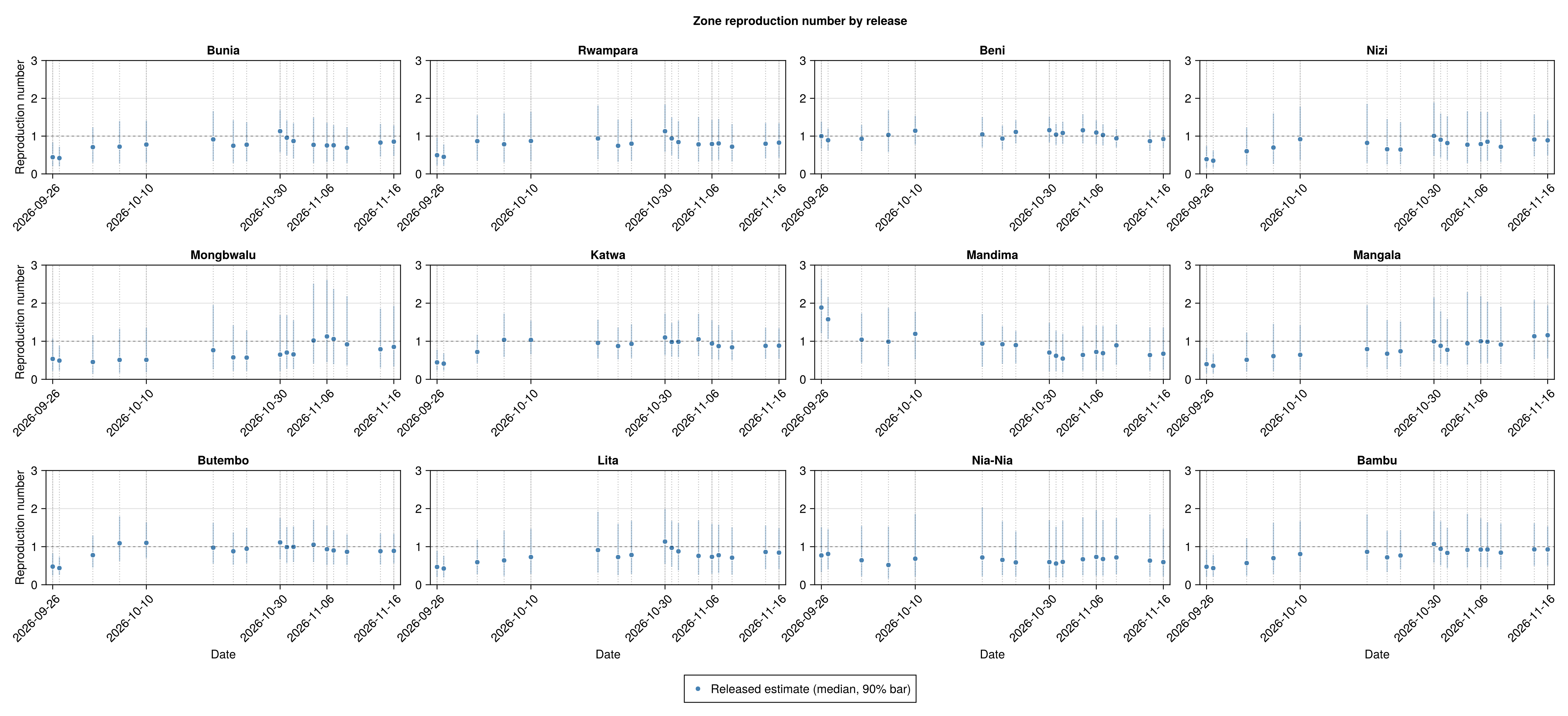
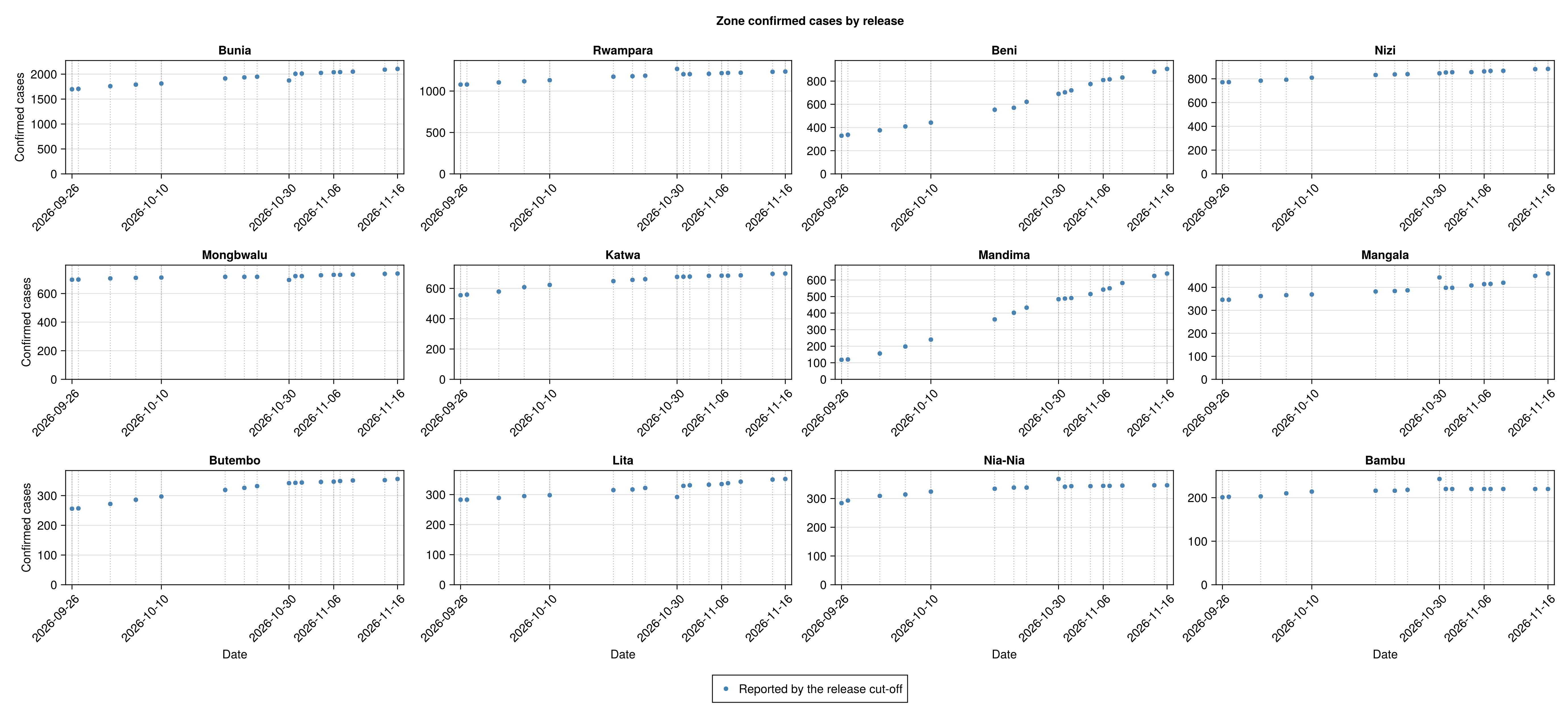
How the reproduction number and confirmed cases of the twelve zones with most confirmed cases to date have moved as releases accrued, read from the estimates each release published at its own cut-off. A zone that a release did not estimate has no mark for that release.
Load the per-zone estimates of each release
# Written by `scripts/score_releases.jl` from each release's
# `zone_estimates.csv`, one row per release, zone and quantity, keyed as
# `<province>.<zone>` like the zone model. A missing file reads as an empty
# table, which the figures report as nothing collected.
zone_release_df = _release_data(
    joinpath("zone", "released_estimates.csv"),
    (;
        release = String, date = Date, area = String, label = String,
        province = String, patch = String, quantity = String,
        median = Float64, lo90 = Float64, hi90 = Float64,
    )
)
# The twelve zones with most confirmed cases in the current data, among
# those any release estimated.
_release_zones = let keys = Set(zone_release_df.area),
        order = sortperm(zone_inputs.cumulative; rev = true)

    first(
        [zone_inputs.zone_keys[z] for z in order if zone_inputs.zone_keys[z] in keys],
        12
    )
end
_release_zone_titles = Dict(zip(zone_inputs.zone_keys, zone_inputs.zone_labels))
_zone_release_groups(q) = area_evolution_groups(
    zone_release_df, q; areas = _release_zones, labels = _release_zone_titles
)
_no_zone_release_note = "No releases scored yet. This fills in as releases accumulate."
zone_rt_release_fig = plot_evolution_by_group(
    _zone_release_groups("R_T");
    ylabel = "Reproduction number",
    title = "Zone reproduction number by release",
    released_label = "Released estimate", marks_label = "median, 90% bar",
    refline = 1.0, ymax = 3.0, ncols = 4,
    empty_note = _no_zone_release_note
);
zone_cases_release_fig = plot_evolution_by_group(
    _zone_release_groups("cases");
    ylabel = "Confirmed cases",
    title = "Zone confirmed cases by release",
    released_label = "Reported by the release cut-off", marks_label = "",
    shared_yrange = false, ncols = 4, empty_note = _no_zone_release_note
);
Reproduction number by release
Confirmed cases by release
Saving zone in-sample outputs
Write the summary bullets
# The bullets under the summary heading at the top of the page. They read
# the calibration table built further down, so they are written here and
# read back when the site is assembled.
evaluation_insample_zone_summary = let
    fmt(x) = ismissing(x) || !isfinite(x) ? "n/a" :
        string(round(x; digits = 2))
    # The per-patch rows only: the table's "All zones" rows pool them and
    # would be counted twice.
    fitted = filter(
        r -> isfinite(r["Bias"]) && !startswith(r["Stream"], "All zones"),
        zone_calibration_table
    )
    worst = first(
        sort(fitted, "Bias"; by = abs, rev = true), min(3, size(fitted, 1))
    )[!, "Stream"]
    low = first(sort(fitted, "90% coverage"), min(1, size(fitted, 1)))
    overall = [
        isempty(worst) ? nothing :
            string(
                "- **Least well reproduced:** ", join_names(worst),
                length(worst) == 1 ? " has" : " have",
                " the largest absolute bias."
            ),
        string(
            "- **Coverage:** ", count(>=(0.8), fitted[!, "90% coverage"]),
            " of ", size(fitted, 1),
            " composition rows have 90% coverage of at least 0.8",
            size(low, 1) == 0 ? "." :
                string(
                    "; the lowest is ", low[1, "Stream"], " at ",
                    fmt(low[1, "90% coverage"]), "."
                )
        ),
    ]
    # The province whose zone-stage level sits furthest from the joint's
    # over the last fortnight.
    recent = filter(
        r -> r["Province"] != "All provinces" &&
            r["Week ending"] >= maximum(zone_level_table[!, "Week ending"]) -
            Day(7),
        zone_level_table
    )
    if size(recent, 1) > 0
        far = recent[argmax(abs.(recent[!, "Ratio"] .- 1)), :]
        push!(
            overall, string(
                "- **Province levels:** over the last two weeks the zone ",
                "stage's infections are within ",
                fmt(100 * abs(far["Ratio"] - 1)),
                "% of the joint model's in every province, the furthest ",
                "being ", far["Province"], "."
            )
        )
    end
    # One row per province and composition.
    rows = Dict(r["Stream"] => r for r in eachrow(zone_calibration_table))
    cells = [
        (PROVINCE_LABELS[p], what, label) for p in 1:N_PATCHES
            for (what, label) in
            (("cases", "Confirmed cases"), ("deaths", "Confirmed deaths"))
    ]
    value(label, what, col) = let r = get(
            rows, string(label, " (", what, ")"), nothing
        )
        r === nothing ? missing : r[col]
    end
    table = DataFrame(
        "Province" => [c[1] for c in cells],
        "Stream" => [c[3] for c in cells],
        "Bias" => [finite_round(value(c[1], c[2], "Bias")) for c in cells],
        "90% coverage" => [
            finite_round(value(c[1], c[2], "90% coverage")) for c in cells
        ],
        "Cells" => [value(c[1], c[2], "Vintages") for c in cells],
    )
    join(
        [
            join(filter(!isnothing, overall), "\n"),
            markdown_table(table; missing_text = "n/a"),
        ],
        "\n\n"
    )
end
dashboard_dir = joinpath(
    pkgdir(BVDOutbreakSize), "docs", "src", "summary_assets"
)
mkpath(dashboard_dir)
write(
    joinpath(dashboard_dir, "evaluation_insample_zone.md"),
    evaluation_insample_zone_summary
);