Forecast evaluation
How the forecasts on the forecasts page have scored against the data that arrived afterwards. How the outbreak-size and reproduction-number estimates moved from release to release is on the in-sample checks page. Scoring is the continuous ranked probability score against a persistence baseline, defined in the forecast scoring Methods section. The same scoring by province is on the province forecast evaluation page and by health zone on the health-zone forecast evaluation page.
Load packages, data and fitted chains
# Shared setup: packages, observations and the fit registry. See
# `docs/pages/_setup.jl`.
using BVDOutbreakSize
include(joinpath(pkgdir(BVDOutbreakSize), "docs", "pages", "_setup.jl"))
validation_forecast_from (generic function with 1 method)# The fits this page reads, loaded from the cache here.
chn_joint = load_fit("joint")
frozen_lastweek = load_fit("frozen_validation")
frozen_lastweek_streams = frozen_validation_stream_fits();Summary
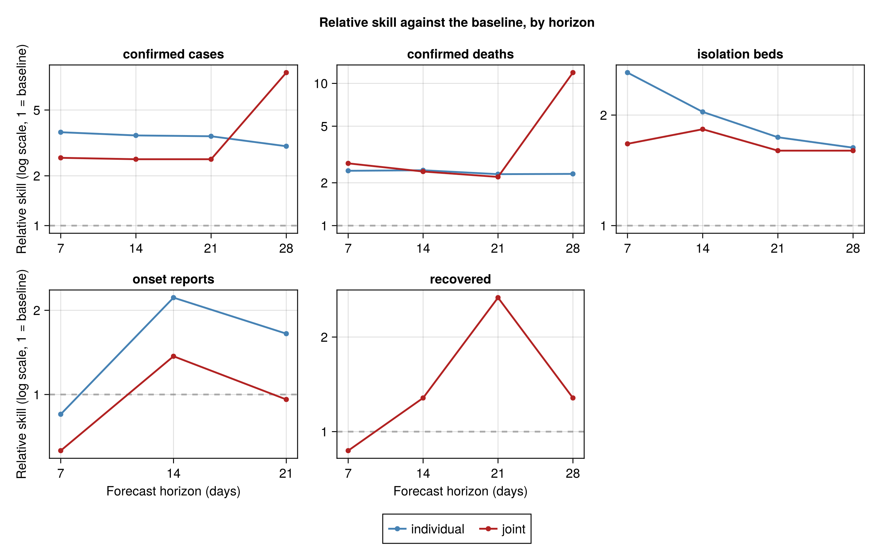
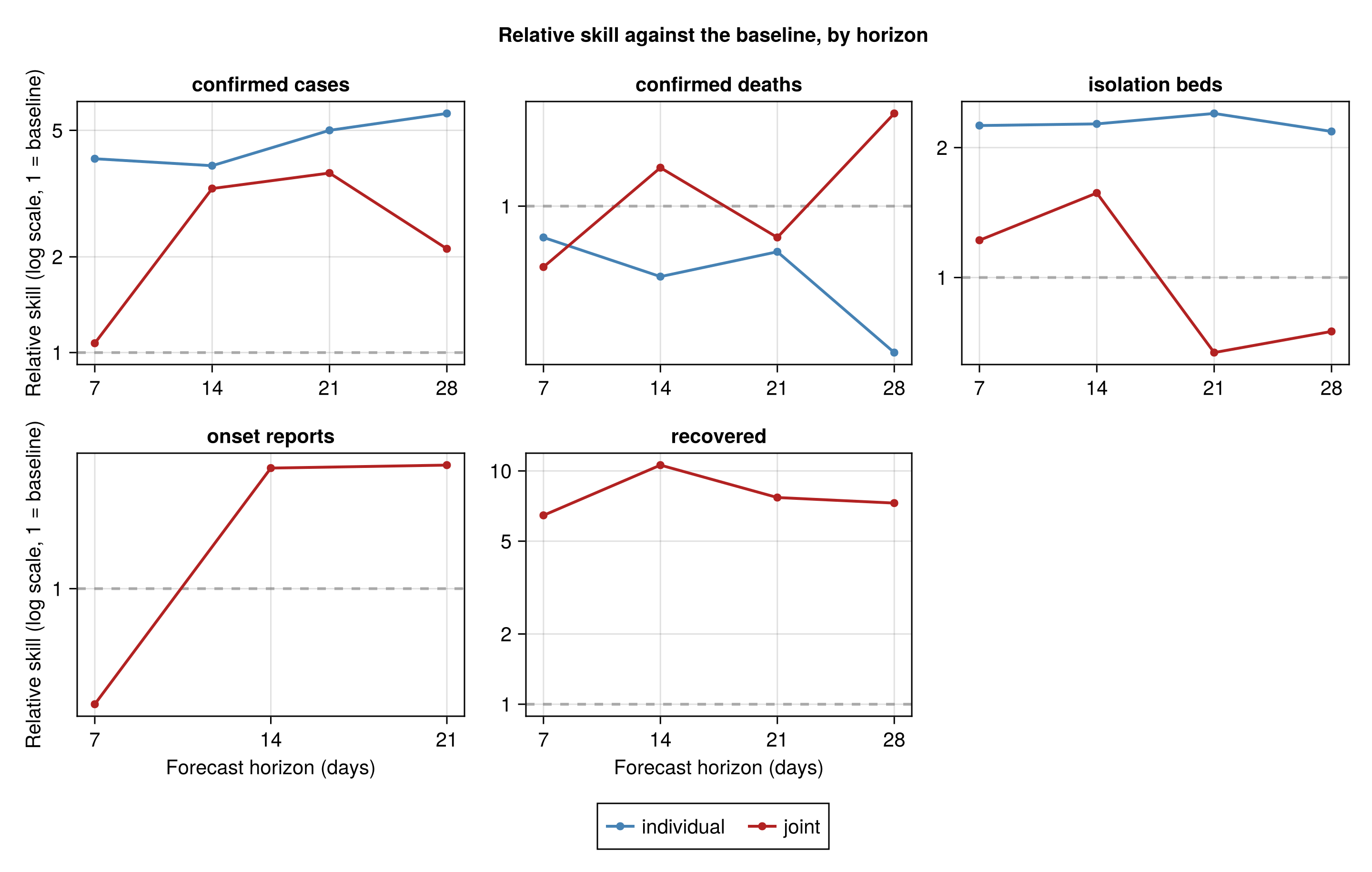
The overall bullets come first, then each stream's own scores, from the sections below. Relative skill is the model's CRPS over the persistence baseline's, so a value below one beats the baseline. Coverage is the fraction of forecasts whose observed value falls inside the 90% predictive interval, nominally 0.9.
Joint model across releases: beat the baseline on 1 of 5 streams.
Frozen joint model: beat the baseline on 1 of 5 streams.
Across releases
confirmed cases: relative skill 5.24, 90% coverage 0.87, bias 0.39 over 143 forecasts.
confirmed deaths: relative skill 6.86, 90% coverage 0.85, bias 0.08 over 141 forecasts.
isolation beds: relative skill 1.67, 90% coverage 0.96, bias 0.14 over 138 forecasts.
onset reports: relative skill 0.91, 90% coverage 0.96, bias -0.04 over 27 forecasts.
recovered: relative skill 1.61, 90% coverage 1.0, bias 0.12 over 45 forecasts.
Frozen fits
confirmed cases: relative skill 2.39, 90% coverage 0.77, bias 0.31 over 308 forecasts.
confirmed deaths: relative skill 1.02, 90% coverage 0.83, bias 0.06 over 252 forecasts.
isolation beds: relative skill 0.87, 90% coverage 0.98, bias 0.12 over 273 forecasts.
onset reports: relative skill 1.03, 90% coverage 0.9, bias -0.16 over 30 forecasts.
recovered: relative skill 7.77, 90% coverage 0.62, bias 0.53 over 133 forecasts.
Forecast validation
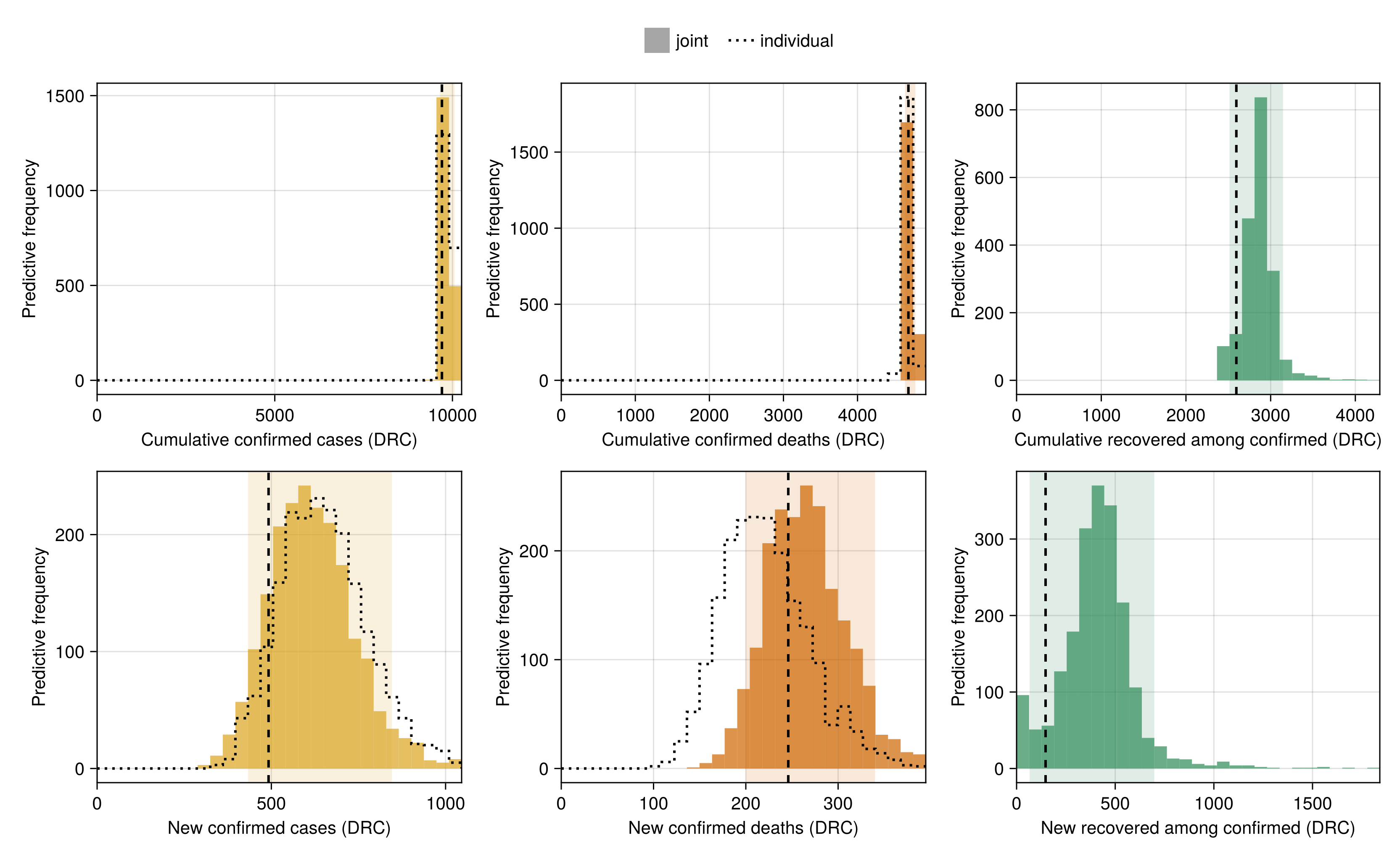
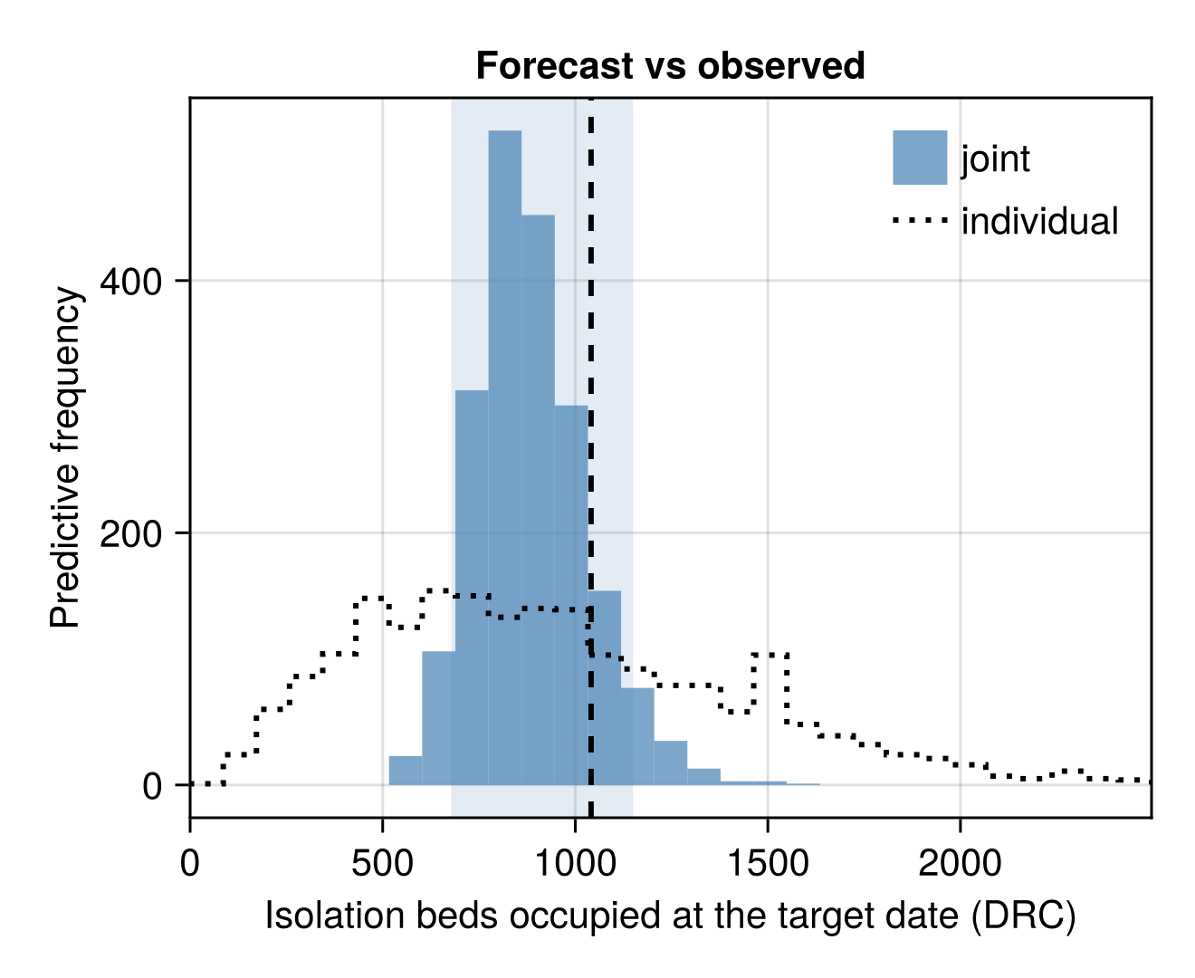
How last week's forecast held up against the data since observed, from the frozen refit in forecast-versus-frozen evaluation. Only the streams the situation reports still update are validated, since a stopped stream repeats its last total and leaves nothing to score. The projected bed occupancy is scored against the beds held a week later, but this check is weak at a one-week-back freeze. The reported occupancy rate starts only on 9 June, so the capacity has no implied-capacity anchor and rides its random walk back to the freeze date.
Fit one week back and validate the one-week-ahead forecast
# frozen_lastweek and frozen_lastweek_streams are computed in the setup
# block above, and `validation_forecast_from` is defined there.
validation_forecast = validation_forecast_from("frozen_validation");

# Each frozen individual (single-stream) fit's own one-week-ahead new-count
# forecast at the same cut-off as `frozen_lastweek`, from
# [`forecast_stream`](@ref) (the same per-stream forecaster
# `stream_forecasts.csv` uses), so the validation plots below can show the
# individual fit alongside the joint rather than the joint alone. Recovered
# has no individual fit and is absent here, as it is throughout this report.
# Only the still-reported streams are fitted at the validation cut-off, so
# a stream the situation reports have stopped updating is absent from
# `frozen_lastweek_streams` and carries no individual series here.
function _validation_individual_new(sid, stream::Symbol)
    haskey(frozen_lastweek_streams, sid) || return nothing
    return Float64.(
        forecast_stream(
            fit_forecast("frozen_validation_$sid"), stream; horizon = 7
        )
    )
end
validation_individual = NamedTuple(
    k => v
        for (k, v) in pairs(
            (;
                cases_new = _validation_individual_new(
                    "cases", :reported_cases
                ),
                deaths_new = _validation_individual_new(
                    "deaths", :suspected_deaths
                ),
                confirmed_new = _validation_individual_new(
                    "confirmed", :confirmed_cases
                ),
                confirmed_deaths_new = _validation_individual_new(
                    "confirmed_deaths", :confirmed_deaths
                ),
            )
        )
        if !isnothing(v)
)
# The frozen individual (treatment-only) fit's own bed-occupancy forecast.
# `nothing` when the beds have stopped being reported, so the treatment fit
# is absent; the bed panel then draws the joint alone.
validation_individual_isolation = haskey(frozen_lastweek_streams, "treatment") ?
    Float64.(
        forecast_stream(
            fit_forecast("frozen_validation_treatment"), :isolation_beds;
            horizon = 7
        )
    ) : nothing

# The observed beds at the current cut-off (the forecast target), so the
# frozen-fit bed forecast is scored against what the beds actually held.
# Held back once the beds stop being reported, since the last count would
# then be carried forward rather than observed at the target date.
_obs_beds = stream_reporting(obs, :isolation_beds) ?
    obs.isolation_history.counts[end] : missing
# Same observed/baseline keying as the plot below, so the table covers every
# fitted count stream (cumulative and new-count rows) plus the bed level.
# A harmonisation-break day between the frozen cut-off and the current one
# puts records into the confirmed cumulative that were never notified in that
# week, so the new-count truth carries a step the forecast was never
# predicting. Take it out, the same correction `score_releases.jl` applies.
# Grid days are relative to a seeding date fixed by the genetic tmrca, so the
# frozen fit's own `n` and the current `obs.n` index the same grid.
validation_breaks = (
    confirmed_cum = confirmed_break_correction(
        obs, frozen_lastweek.o.n, obs.n
    ),
    confirmed_deaths_cum = confirmed_break_correction(
        obs, frozen_lastweek.o.n, obs.n; deaths = true
    ),
)

# Observed cumulative at the target date per stream, keyed by the forecast's
# cumulative column; `baseline` is each stream's origin cumulative (the
# frozen cut-off), so the new count is scored against observed minus origin,
# less any harmonisation the window carries (see `validation_breaks`). Both
# the table and the plot below take the still-reported streams
# (`reporting_cum_cols`, from the setup block): a stream the situation
# reports have stopped updating has an origin and a target reading the same
# repeated total, so its cumulative truth is stale and its new-count truth is
# a guaranteed zero.
validation_observed = (
    cases_cum = obs.reported_cases,
    deaths_cum = obs.total_deaths,
    confirmed_cum = obs.confirmed_cases,
    confirmed_deaths_cum = obs.confirmed_deaths,
    recovered_cum = obs.recovered_cases,
)
validation_baseline = (
    cases_cum = frozen_lastweek.o.reported_cases,
    deaths_cum = frozen_lastweek.o.total_deaths,
    confirmed_cum = frozen_lastweek.o.confirmed_cases,
    confirmed_deaths_cum = frozen_lastweek.o.confirmed_deaths,
    recovered_cum = frozen_lastweek.o.recovered_cases,
)

validation_table = forecast_vs_truth(
    validation_forecast;
    observed = keep_streams(validation_observed, reporting_cum_cols),
    baseline = keep_streams(validation_baseline, reporting_cum_cols),
    breaks = validation_breaks,
    isolation = _obs_beds
);
Forecast-versus-observed validation table
| Stream | Quantity | Observed | Lower 90% | Lower 60% | Lower 30% | Upper 30% | Upper 60% | Upper 90% | Within 90% PI |
|---|---|---|---|---|---|---|---|---|---|
| DRC confirmed cases | cumulative by T+7 | 9704 | 9645 | 9725 | 9775 | 9871 | 9925 | 10058 | yes |
| DRC confirmed cases | new this week | 492 | 433 | 513 | 563 | 659 | 713 | 846 | yes |
| DRC confirmed deaths | cumulative by T+7 | 4687 | 4641 | 4670 | 4688 | 4720 | 4742 | 4781 | yes |
| DRC confirmed deaths | new this week | 246 | 200 | 229 | 247 | 279 | 301 | 340 | yes |
| DRC recovered among confirmed | cumulative by T+7 | 2595 | 2514 | 2728 | 2808 | 2910 | 2969 | 3146 | yes |
| DRC recovered among confirmed | new this week | 147 | 66 | 280 | 360 | 462 | 521 | 698 | yes |
| DRC isolation beds | occupancy at T+7 | 1041 | 678 | 766 | 820 | 922 | 989 | 1150 | yes |
Forecast-versus-observed plot
validation_fig = plot_forecast_vs_truth(
    validation_forecast;
    observed = keep_streams(validation_observed, reporting_cum_cols),
    baseline = keep_streams(validation_baseline, reporting_cum_cols),
    breaks = validation_breaks,
    individual = keep_streams(validation_individual, reporting_cum_cols)
);
Bed forecast-versus-observed plot
validation_beds_fig = plot_forecast_beds_vs_truth(
    validation_forecast;
    isolation = _obs_beds, individual = validation_individual_isolation
);
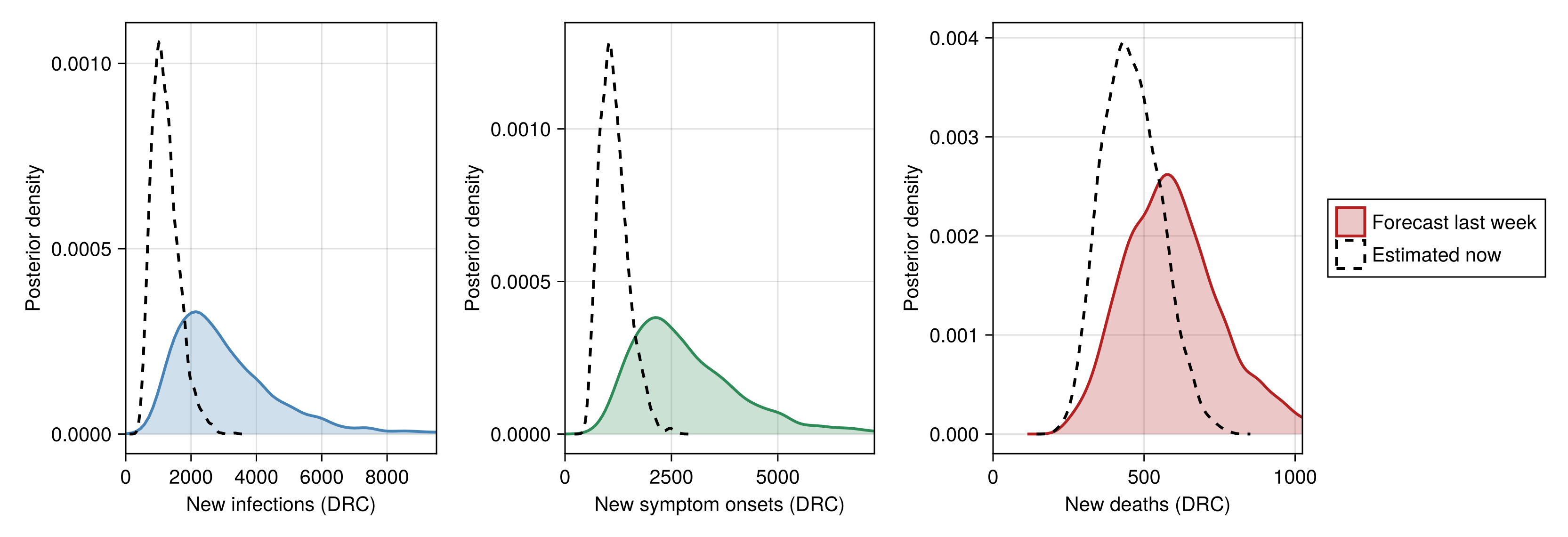
Forecast-versus-now latent plot
# Current fit's draws of the new latent counts over the past week, the last
# seven days of each cumulative-trajectory deterministic.
function _now_new(chn, key)
    mat = chn[key]
    trajs = [collect(v) for v in vec(collect(mat))]
    return Float64[t[end] - t[max(1, length(t) - 7)] for t in trajs]
end
now_latent = (;
    infections_new = _now_new(chn_joint, :cumulative_infections),
    onsets_new = _now_new(chn_joint, :cumulative_onsets),
    deaths_latent_new = _now_new(chn_joint, :cumulative_expected_deaths),
)

validation_latent_fig = plot_forecast_vs_truth_latent(
    validation_forecast; now = now_latent
);
Streams no longer reported
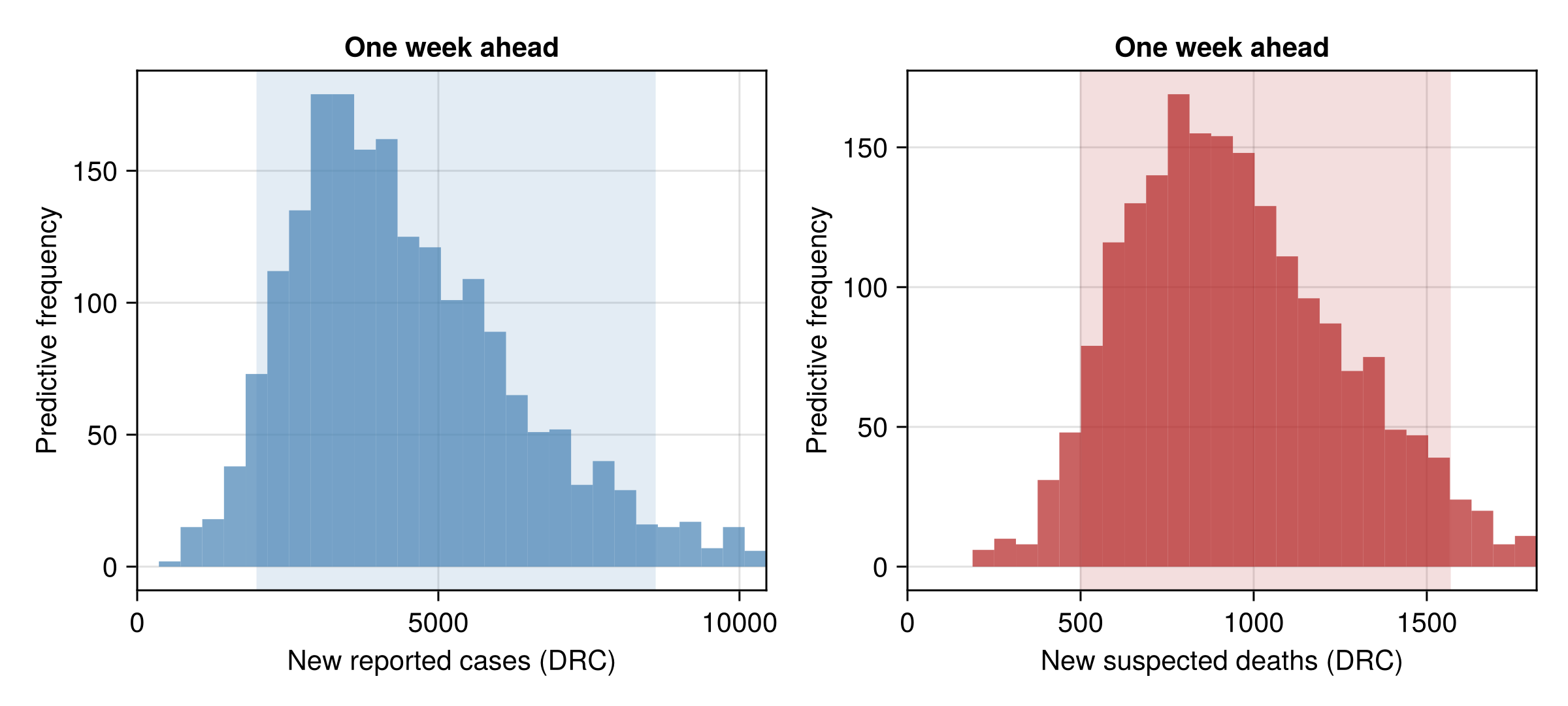
Forecast for the streams no longer reported
# The last-reported date per stopped stream, and the frozen fit's own
# projection for them. `plot_forecast` draws a panel per new-count column
# the frame carries, so passing the stopped streams' columns alone gives the
# projection without the fabricated truth rule the validation figure would
# otherwise draw against a repeated total.
validation_stopped_streams = let s = stream_report_status(obs),
        ids = [stream_id(c) for c in stopped_cum_cols]

    keep = [r.stream in ids for r in eachrow(s)]
    DataFrame(
        "Stream" => s[keep, :label],
        "Last reported" => s[keep, :last_date]
    )
end
_stopped_new_cols = [
    c
        for c in new_cols(stopped_cum_cols)
        if c in propertynames(validation_forecast)
]
validation_stopped_fig = plot_forecast(
    validation_forecast[!, _stopped_new_cols]
);| Stream | Last reported |
|---|---|
| Suspected cases | 2026-05-26 |
| Suspected deaths | 2026-05-26 |
Forecast scoring across releases
Every release's saved one- to four-week-ahead forecast is scored against the data observed since, against a persistence baseline and, where one exists, the stream's own individual fit. The tables in this section are the joint model's, one row per stream. Recovered has no individual fit of its own, so it is compared with the baseline only. Reported cases and suspected deaths stopped being updated partway through the outbreak, and the exports detection series is anchored to an earlier cut-off. Exports therefore has no scored forecast, and reported cases and suspected deaths each rest on a single matched forecast.
Only a minority of the daily releases examined contribute a row, each a reconstruction of an earlier model version rather than the current fit. Only the newest few releases carry the current model's individual-stream forecasts. Each row shows the number of matched forecasts it rests on, from one to a handful.
Four things are excluded from the scores, each for a stated reason rather than for scoring badly:
One whole reconstruction (
results-v1.6.0), whose chain forecasts a near-zero median at every horizon and stream with an occasional five- or six-digit upper tail, the signature of a chain that failed to sample.In the frozen section only, the confirmed-death rows of the fourteen frozen reconstructions cut between 16 July and 15 August 2026. Their forecaster floored that stream at zero, giving a one-week median of zero against an observed 250 to 370.
An onset window containing a vintage whose reread total falls, since its increment is not what the situation reports added.
A stream that carries no persistence baseline, which is what makes a window scoreable at all.
Nothing is dropped from the archive itself, and the score and overlay files in the data directory record everything that was scored.
The symptom-onset stream is scored on the new reported count each vintage adds, because every vintage rereads the whole figure. Its printed total therefore moves with the scan error as well as with late reporting, and on fourteen vintages the reread total falls. A window containing a falling vintage is left unscored, as the province scores do for a window holding a harmonisation-break day. This bites hardest at the longer horizons: the frozen onset row keeps three of its twenty-nine windows, all at one week, and the cross-release row six of thirty-eight. Read the onset row's skill against the baseline rather than its coverage, and as resting on a handful of windows.
Load and summarise the cross-release forecast scores
forecast_scores_df = _release_data(
    "forecast_scores.csv",
    (;
        release = String, made_date = Date, stream = String, horizon = Int,
        target_date = Date, fit = String, crps = Float64,
        log_crps = Float64, dispersion = Float64, overprediction = Float64,
        underprediction = Float64, coverage_50 = Float64,
        coverage_90 = Float64,
        bias = Float64, n_samples = Int,
        log_rel_to_baseline = Float64,
    )
)
forecast_overlay_df = _release_data(
    "forecast_overlay.csv",
    (;
        release = String, made_date = Date, stream = String, horizon = Int,
        target_date = Date, fit = String, observed = Float64,
        median = Float64, lo30 = Float64, hi30 = Float64, lo60 = Float64,
        hi60 = Float64, lo90 = Float64, hi90 = Float64,
    )
)
# The digitised onset triangle's own per-vintage total, as calendar dates,
# and the windows it makes unscoreable. A vintage that rereads the figure
# lower gives a window an increment the reports did not add, so the window
# is dropped from the scores and the overlay alike (see
# `drop_rescanned_onset_windows`). The current triangle is used to judge
# every release, since the scored truth is read off this one series.
_onset_vintage_dates = grid_date.(obs.onset_report_history.days)
_onset_vintage_totals = obs.onset_report_history.counts
_drop_rescanned(tbl) = drop_rescanned_onset_windows(
    tbl; vintage_dates = _onset_vintage_dates,
    vintage_totals = _onset_vintage_totals
)
forecast_scores_df = _drop_rescanned(forecast_scores_df)
forecast_overlay_df = _drop_rescanned(forecast_overlay_df)

# One row per (stream, fit) pooled over every horizon and release. The
# by-horizon and by-release detail tables carry the same columns at a finer
# grain (see src/scoring.jl). Every fit is kept here, since the
# relative-skill figure below compares the roles against each other. The
# tables rendered in this section select the joint role, and the individual
# fits are tabulated in their own section.
forecast_score_overview_table = forecast_score_overview(forecast_scores_df)
forecast_score_by_horizon_table = forecast_score_by_horizon(forecast_scores_df)
forecast_score_by_release_table = forecast_score_by_release(forecast_scores_df)

joint_score_overview_table = select_fit_role(
    forecast_score_overview_table, "joint"
)
joint_score_by_horizon_table = select_fit_role(
    forecast_score_by_horizon_table, "joint"
)
# The trailing `;` on this last assignment matters: without it, this whole
# setup chunk's last statement (the DataFrame it assigns) is Literate's
# implicitly displayed "result" for the chunk, on top of the deliberate
# display further down -- and a bare DataFrame is html-showable, so it
# goes out as a second, undisplayed-in-source `@raw html` block that (for
# a table this size) can itself hit the PCRE limit described above.
joint_score_by_release_table = select_fit_role(
    forecast_score_by_release_table, "joint"
);| stream | fit | n | crps | rel_to_baseline | log_crps | log_rel_to_baseline | rel_to_individual | log_rel_to_individual | dispersion | overprediction | underprediction | coverage_50 | coverage_90 | bias |
|---|---|---|---|---|---|---|---|---|---|---|---|---|---|---|
| confirmed cases | joint | 143 | 747.24 | 5.24 | 0.223 | 1.98 | 0.69 | 0.65 | 610.89 | 135.7 | 0.65 | 0.6 | 0.87 | 0.39 |
| confirmed deaths | joint | 141 | 666.86 | 6.86 | 0.383 | 2.55 | 0.92 | 0.94 | 562.61 | 43.33 | 60.92 | 0.34 | 0.85 | 0.08 |
| isolation beds | joint | 138 | 95.84 | 1.67 | 0.111 | 1.53 | 0.88 | 0.72 | 55.78 | 30.17 | 9.88 | 0.64 | 0.96 | 0.14 |
| onset reports | joint | 27 | 121.43 | 0.91 | 0.189 | 0.82 | 0.65 | 0.62 | 70.92 | 12.91 | 37.59 | 0.63 | 0.96 | -0.04 |
| recovered | joint | 45 | 58.52 | 1.61 | 0.146 | 1.06 | 45.67 | 9.39 | 3.46 | 0.82 | 1 | 0.12 |
forecast_relative_skill_fig = plot_forecast_relative_skill(
    forecast_score_by_horizon_table
);
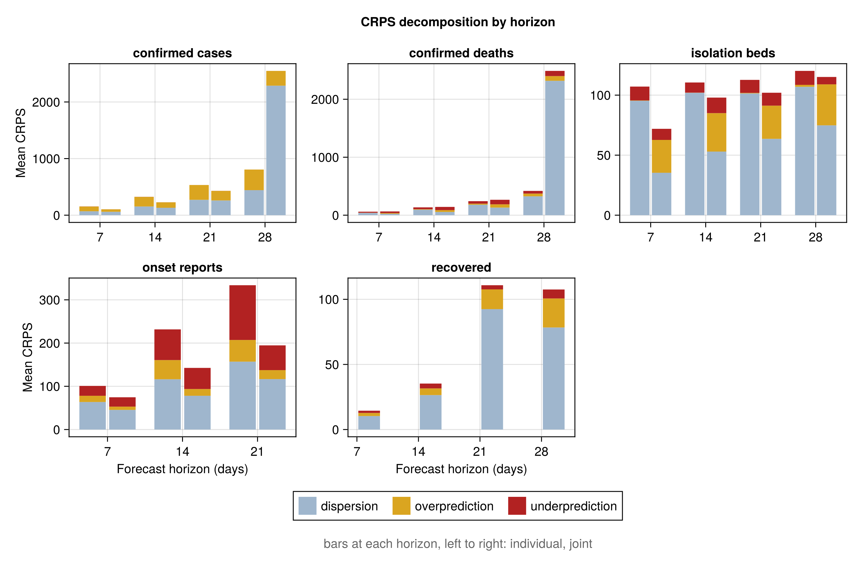
forecast_crps_by_horizon_fig = plot_forecast_crps_by_horizon(
    forecast_score_by_horizon_table
);
Scores by horizon
| stream | horizon | fit | n | crps | rel_to_baseline | log_crps | log_rel_to_baseline | rel_to_individual | log_rel_to_individual | dispersion | overprediction | underprediction | coverage_50 | coverage_90 | bias |
|---|---|---|---|---|---|---|---|---|---|---|---|---|---|---|---|
| confirmed cases | 7 | joint | 39 | 104.69 | 2.57 | 0.217 | 2.55 | 0.59 | 0.59 | 59.99 | 44.01 | 0.68 | 0.59 | 0.87 | 0.4 |
| confirmed cases | 14 | joint | 38 | 228.3 | 2.52 | 0.217 | 2.27 | 0.62 | 0.63 | 131.02 | 96.59 | 0.69 | 0.63 | 0.87 | 0.36 |
| confirmed cases | 21 | joint | 35 | 430.63 | 2.52 | 0.217 | 1.78 | 0.66 | 0.66 | 260.5 | 169.14 | 0.99 | 0.63 | 0.86 | 0.38 |
| confirmed cases | 28 | joint | 31 | 2549.17 | 8.42 | 0.247 | 1.55 | 0.76 | 0.74 | 2287.78 | 261.22 | 0.17 | 0.55 | 0.9 | 0.43 |
| confirmed deaths | 7 | joint | 39 | 64.66 | 2.74 | 0.405 | 3.98 | 1.07 | 0.97 | 23.95 | 12.64 | 28.07 | 0.41 | 0.79 | 0.04 |
| confirmed deaths | 14 | joint | 37 | 142.98 | 2.4 | 0.361 | 2.83 | 1.03 | 0.95 | 55.71 | 32.04 | 55.24 | 0.32 | 0.84 | 0.08 |
| confirmed deaths | 21 | joint | 34 | 266.02 | 2.2 | 0.373 | 2.23 | 0.95 | 0.94 | 131.07 | 56.42 | 78.53 | 0.26 | 0.85 | 0.09 |
| confirmed deaths | 28 | joint | 31 | 2489.39 | 11.91 | 0.393 | 1.8 | 0.82 | 0.89 | 2318.6 | 81.07 | 89.72 | 0.35 | 0.94 | 0.11 |
| isolation beds | 7 | joint | 37 | 71.95 | 1.67 | 0.086 | 1.57 | 0.67 | 0.55 | 35.34 | 27.37 | 9.24 | 0.54 | 0.95 | 0.19 |
| isolation beds | 14 | joint | 36 | 97.96 | 1.83 | 0.112 | 1.67 | 0.92 | 0.75 | 53 | 32.01 | 12.95 | 0.53 | 0.97 | 0.13 |
| isolation beds | 21 | joint | 34 | 102 | 1.6 | 0.117 | 1.45 | 0.95 | 0.79 | 63.61 | 27.64 | 10.75 | 0.76 | 0.97 | 0.1 |
| isolation beds | 28 | joint | 31 | 115.14 | 1.6 | 0.134 | 1.48 | 1 | 0.84 | 74.84 | 34.16 | 6.14 | 0.77 | 0.97 | 0.14 |
| onset reports | 7 | joint | 13 | 74.62 | 0.63 | 0.221 | 0.67 | 0.74 | 0.63 | 45.39 | 7.63 | 21.6 | 0.69 | 0.92 | 0.02 |
| onset reports | 14 | joint | 8 | 142.57 | 1.37 | 0.166 | 1.37 | 0.62 | 0.62 | 78.1 | 15.62 | 48.85 | 0.62 | 1 | -0.06 |
| onset reports | 21 | joint | 6 | 194.67 | 0.96 | 0.15 | 0.93 | 0.58 | 0.58 | 116.67 | 20.77 | 57.23 | 0.5 | 1 | -0.15 |
| recovered | 7 | joint | 14 | 14.47 | 0.87 | 0.122 | 0.96 | 10.37 | 2.37 | 1.73 | 0.86 | 1 | 0.02 | ||
| recovered | 14 | joint | 13 | 35.3 | 1.28 | 0.133 | 1.17 | 26.46 | 5.13 | 3.72 | 0.85 | 1 | 0.16 | ||
| recovered | 21 | joint | 11 | 110.82 | 2.67 | 0.169 | 1.28 | 92.48 | 15.16 | 3.19 | 0.82 | 1 | 0.16 | ||
| recovered | 28 | joint | 7 | 107.56 | 1.28 | 0.183 | 0.86 | 78.39 | 22.28 | 6.89 | 0.71 | 1 | 0.18 |
forecast_skill_by_cutoff_fig = plot_forecast_skill_by_cutoff(
    forecast_score_by_release_table;
    title = "Relative skill against the baseline, by release"
);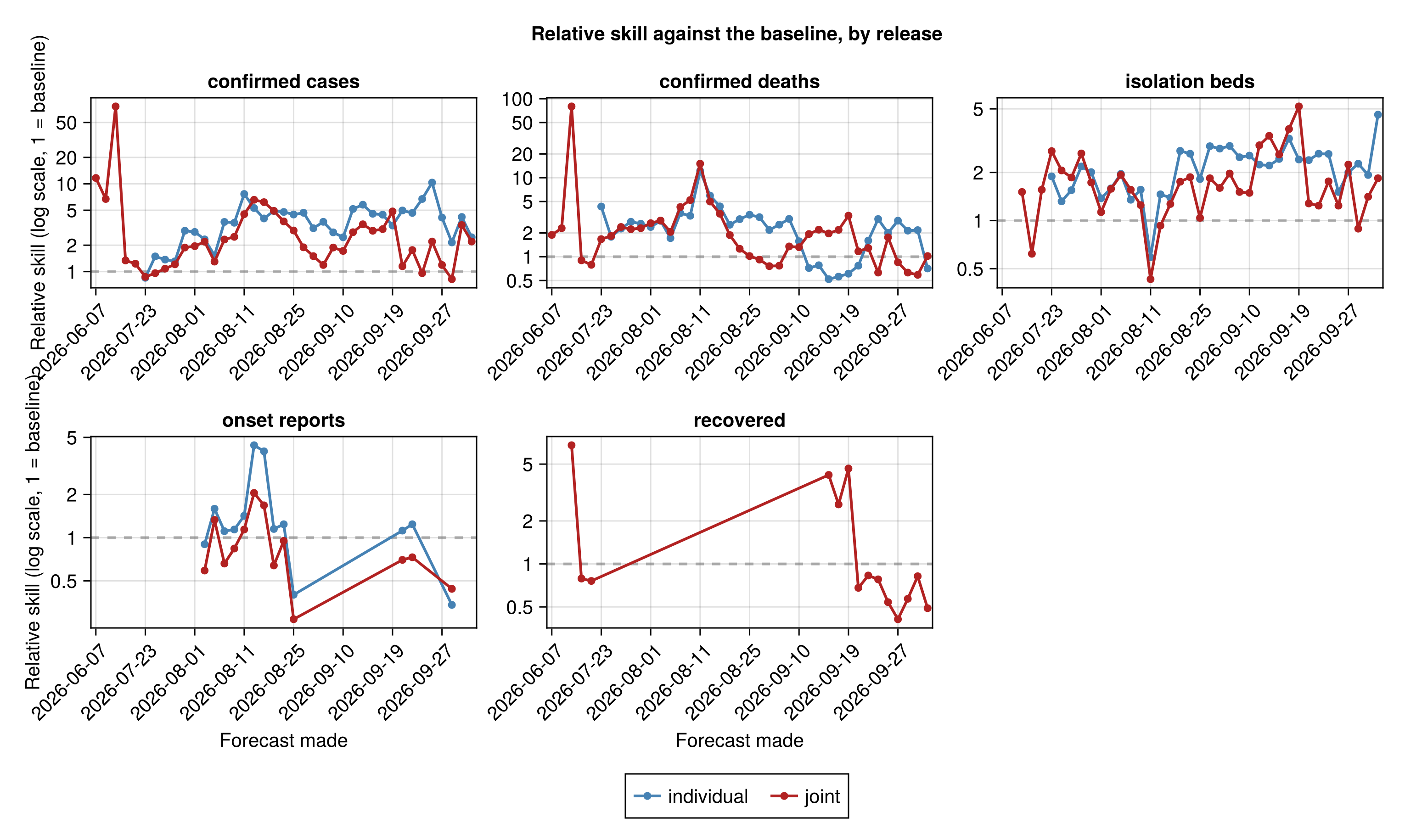
Scores by release
| made_date | stream | fit | n | crps | rel_to_baseline | log_crps | log_rel_to_baseline | rel_to_individual | log_rel_to_individual | dispersion | overprediction | underprediction | coverage_50 | coverage_90 | bias |
|---|---|---|---|---|---|---|---|---|---|---|---|---|---|---|---|
| 2026-06-07 | confirmed cases | joint | 2 | 363.91 | 11.66 | 0.913 | 9.51 | 341.06 | 22.86 | 0 | 1 | 1 | 0.17 | ||
| 2026-06-10 | confirmed cases | joint | 3 | 534.87 | 6.72 | 0.791 | 5.07 | 435.67 | 99.2 | 0 | 1 | 1 | 0.27 | ||
| 2026-07-01 | confirmed cases | joint | 4 | 15862.78 | 76.2 | 0.583 | 2.9 | 15377.31 | 485.47 | 0 | 0 | 1 | 0.66 | ||
| 2026-07-06 | confirmed cases | joint | 4 | 421.28 | 1.34 | 0.269 | 0.97 | 311.85 | 109.43 | 0 | 0.5 | 1 | 0.49 | ||
| 2026-07-08 | confirmed cases | joint | 4 | 390.98 | 1.23 | 0.253 | 0.96 | 239.5 | 151.47 | 0 | 0.25 | 1 | 0.52 | ||
| 2026-07-23 | confirmed cases | joint | 4 | 335.57 | 0.87 | 0.169 | 0.66 | 1.02 | 0.82 | 299.27 | 35.68 | 0.62 | 1 | 1 | 0.13 |
| 2026-07-25 | confirmed cases | joint | 4 | 222.5 | 0.96 | 0.134 | 0.95 | 0.64 | 0.63 | 218.04 | 4.46 | 0 | 1 | 1 | 0.07 |
| 2026-07-26 | confirmed cases | joint | 4 | 235.69 | 1.08 | 0.141 | 1.07 | 0.79 | 0.67 | 229.65 | 5.68 | 0.36 | 1 | 1 | 0.06 |
| 2026-07-27 | confirmed cases | joint | 4 | 247.97 | 1.21 | 0.142 | 1.03 | 0.93 | 0.83 | 240.08 | 7.88 | 0 | 1 | 1 | 0.11 |
| 2026-07-31 | confirmed cases | joint | 4 | 259.64 | 1.88 | 0.149 | 1.71 | 0.64 | 0.68 | 235.73 | 23.76 | 0.15 | 1 | 1 | 0.13 |
| 2026-08-01 | confirmed cases | joint | 4 | 231.26 | 1.95 | 0.139 | 1.94 | 0.69 | 0.66 | 226.84 | 4.31 | 0.11 | 1 | 1 | 0.05 |
| 2026-08-02 | confirmed cases | joint | 4 | 278.45 | 2.19 | 0.145 | 1.81 | 0.94 | 0.85 | 263.77 | 14.68 | 0 | 1 | 1 | 0.14 |
| 2026-08-03 | confirmed cases | joint | 4 | 247.58 | 1.3 | 0.14 | 0.98 | 0.85 | 0.8 | 237.88 | 9.7 | 0 | 1 | 1 | 0.08 |
| 2026-08-04 | confirmed cases | joint | 4 | 221.56 | 2.32 | 0.133 | 2.26 | 0.63 | 0.69 | 220.7 | 0.86 | 0 | 1 | 1 | 0.03 |
| 2026-08-07 | confirmed cases | joint | 4 | 213.54 | 2.49 | 0.14 | 2.03 | 0.69 | 0.73 | 209.76 | 0 | 3.78 | 1 | 1 | -0.09 |
| 2026-08-11 | confirmed cases | joint | 4 | 197.49 | 4.51 | 0.135 | 3.73 | 0.59 | 0.71 | 191.53 | 0 | 5.97 | 1 | 1 | -0.13 |
| 2026-08-15 | confirmed cases | joint | 4 | 387.77 | 6.58 | 0.193 | 3.83 | 1.24 | 0.91 | 294.02 | 93.75 | 0 | 1 | 1 | 0.37 |
| 2026-08-17 | confirmed cases | joint | 4 | 458.71 | 6.18 | 0.222 | 3.37 | 1.53 | 0.97 | 290.38 | 168.33 | 0 | 0.5 | 1 | 0.46 |
| 2026-08-22 | confirmed cases | joint | 4 | 336.09 | 4.92 | 0.178 | 3.51 | 1 | 0.87 | 228.94 | 107.15 | 0 | 0.75 | 1 | 0.45 |
| 2026-08-24 | confirmed cases | joint | 4 | 246.11 | 3.73 | 0.144 | 3.05 | 0.78 | 0.77 | 118.34 | 127.77 | 0 | 0 | 1 | 0.62 |
| 2026-08-25 | confirmed cases | joint | 4 | 198.57 | 2.94 | 0.12 | 2.6 | 0.66 | 0.65 | 108.48 | 90.1 | 0 | 0 | 1 | 0.56 |
| 2026-08-30 | confirmed cases | joint | 4 | 155.68 | 1.89 | 0.089 | 1.53 | 0.4 | 0.44 | 99.68 | 55.99 | 0 | 0.75 | 1 | 0.38 |
| 2026-08-31 | confirmed cases | joint | 4 | 143.98 | 1.5 | 0.085 | 1.35 | 0.48 | 0.48 | 106.09 | 37.89 | 0 | 1 | 1 | 0.29 |
| 2026-09-01 | confirmed cases | joint | 4 | 113.16 | 1.19 | 0.07 | 1.05 | 0.32 | 0.36 | 97.21 | 15.95 | 0 | 1 | 1 | 0.17 |
| 2026-09-06 | confirmed cases | joint | 4 | 236.66 | 1.88 | 0.141 | 1.8 | 0.67 | 0.65 | 116.22 | 120.44 | 0 | 0.25 | 1 | 0.6 |
| 2026-09-10 | confirmed cases | joint | 4 | 313.88 | 1.72 | 0.205 | 1.57 | 0.7 | 0.78 | 106.15 | 207.73 | 0 | 0 | 1 | 0.79 |
| 2026-09-12 | confirmed cases | joint | 4 | 711.14 | 2.81 | 0.433 | 2.18 | 0.54 | 0.58 | 165.71 | 545.42 | 0 | 0 | 0 | 0.96 |
| 2026-09-13 | confirmed cases | joint | 4 | 720.07 | 3.46 | 0.426 | 2.62 | 0.6 | 0.61 | 207.2 | 512.87 | 0 | 0 | 0 | 0.93 |
| 2026-09-15 | confirmed cases | joint | 4 | 666.04 | 2.92 | 0.431 | 2.17 | 0.64 | 0.66 | 197.5 | 468.54 | 0 | 0 | 0.25 | 0.92 |
| 2026-09-16 | confirmed cases | joint | 4 | 648.53 | 3.05 | 0.419 | 2.31 | 0.68 | 0.68 | 195.04 | 453.49 | 0 | 0 | 0.25 | 0.93 |
| 2026-09-19 | confirmed cases | joint | 4 | 942.36 | 4.85 | 0.585 | 3.55 | 1.45 | 1.21 | 215.69 | 726.67 | 0 | 0 | 0 | 0.97 |
| 2026-09-21 | confirmed cases | joint | 4 | 110.9 | 1.15 | 0.105 | 1.39 | 0.23 | 0.29 | 66.66 | 44.24 | 0 | 0.5 | 1 | 0.53 |
| 2026-09-22 | confirmed cases | joint | 4 | 135.09 | 1.76 | 0.12 | 2.08 | 0.38 | 0.42 | 71.29 | 63.8 | 0 | 0.25 | 1 | 0.61 |
| 2026-09-25 | confirmed cases | joint | 3 | 44.01 | 0.96 | 0.048 | 0.73 | 0.14 | 0.17 | 41.26 | 2.75 | 0 | 1 | 1 | 0.17 |
| 2026-09-26 | confirmed cases | joint | 3 | 81 | 2.2 | 0.105 | 2.29 | 0.21 | 0.28 | 56.24 | 24.76 | 0 | 0.67 | 1 | 0.4 |
| 2026-09-27 | confirmed cases | joint | 3 | 61.01 | 1.19 | 0.067 | 0.86 | 0.29 | 0.35 | 44.78 | 0 | 16.22 | 1 | 1 | -0.35 |
| 2026-10-02 | confirmed cases | joint | 2 | 47.31 | 0.82 | 0.061 | 0.8 | 0.38 | 0.39 | 35.61 | 11.69 | 0 | 1 | 1 | 0.37 |
| 2026-10-06 | confirmed cases | joint | 2 | 109.86 | 3.39 | 0.129 | 2.94 | 0.81 | 0.8 | 47.44 | 62.43 | 0 | 0 | 1 | 0.66 |
| 2026-10-10 | confirmed cases | joint | 1 | 85.95 | 2.2 | 0.156 | 2.06 | 0.9 | 0.9 | 29.23 | 56.72 | 0 | 0 | 1 | 0.77 |
| 2026-06-07 | confirmed deaths | joint | 1 | 41.49 | 1.89 | 0.903 | 2.67 | 36.94 | 0 | 4.55 | 1 | 1 | -0.2 | ||
| 2026-06-10 | confirmed deaths | joint | 2 | 64.93 | 2.3 | 0.735 | 3.15 | 62.7 | 0.99 | 1.24 | 1 | 1 | -0.03 | ||
| 2026-07-01 | confirmed deaths | joint | 4 | 17196 | 80 | 0.549 | 1.2 | 17103.11 | 92.89 | 0 | 1 | 1 | 0.28 | ||
| 2026-07-06 | confirmed deaths | joint | 4 | 197.2 | 0.9 | 0.871 | 2.33 | 110.35 | 0 | 86.85 | 0.25 | 1 | -0.49 | ||
| 2026-07-08 | confirmed deaths | joint | 4 | 177.59 | 0.79 | 0.713 | 1.87 | 84.29 | 0 | 93.3 | 0.25 | 1 | -0.61 | ||
| 2026-07-23 | confirmed deaths | joint | 4 | 271.49 | 1.67 | 0.484 | 2.45 | 0.39 | 1.08 | 172.61 | 0 | 98.88 | 1 | 1 | -0.45 |
| 2026-07-25 | confirmed deaths | joint | 4 | 241.83 | 1.83 | 0.504 | 3.1 | 1.02 | 2.15 | 106.46 | 0 | 135.37 | 0 | 1 | -0.57 |
| 2026-07-26 | confirmed deaths | joint | 4 | 268.46 | 2.38 | 0.554 | 4.33 | 1.05 | 2.17 | 101.59 | 0 | 166.87 | 0 | 1 | -0.64 |
| 2026-07-27 | confirmed deaths | joint | 4 | 249.47 | 2.23 | 0.534 | 3.86 | 0.8 | 2.12 | 109.3 | 0 | 140.17 | 0 | 1 | -0.59 |
| 2026-07-31 | confirmed deaths | joint | 4 | 274.55 | 2.3 | 0.56 | 3.95 | 0.88 | 1.94 | 108.79 | 0 | 165.76 | 0.25 | 1 | -0.58 |
| 2026-08-01 | confirmed deaths | joint | 4 | 313.48 | 2.66 | 0.683 | 4.51 | 1.12 | 2.7 | 94.48 | 0 | 219.01 | 0 | 1 | -0.68 |
| 2026-08-02 | confirmed deaths | joint | 4 | 258.17 | 2.87 | 0.507 | 4.53 | 1.01 | 1.83 | 128.19 | 0 | 129.98 | 0.25 | 1 | -0.53 |
| 2026-08-03 | confirmed deaths | joint | 4 | 268.89 | 2.06 | 0.58 | 3.06 | 1.2 | 2.37 | 123.56 | 0 | 145.33 | 0.25 | 1 | -0.55 |
| 2026-08-04 | confirmed deaths | joint | 4 | 298.06 | 4.26 | 0.656 | 7.97 | 1.2 | 2.32 | 93.54 | 0 | 204.52 | 0 | 1 | -0.67 |
| 2026-08-07 | confirmed deaths | joint | 4 | 366.29 | 5.22 | 0.88 | 8.58 | 1.58 | 2.71 | 76.06 | 0 | 290.23 | 0 | 0.75 | -0.79 |
| 2026-08-11 | confirmed deaths | joint | 4 | 301.17 | 15.06 | 0.798 | 27.69 | 1.23 | 2.37 | 96.55 | 0 | 204.61 | 0 | 1 | -0.7 |
| 2026-08-15 | confirmed deaths | joint | 4 | 205.93 | 5 | 0.32 | 5.15 | 0.84 | 0.94 | 180.35 | 0 | 25.58 | 1 | 1 | -0.26 |
| 2026-08-17 | confirmed deaths | joint | 4 | 202.49 | 3.5 | 0.304 | 3.57 | 0.81 | 1.02 | 187.02 | 0 | 15.47 | 1 | 1 | -0.21 |
| 2026-08-22 | confirmed deaths | joint | 4 | 178.98 | 1.88 | 0.305 | 2.38 | 0.74 | 0.63 | 156.16 | 0 | 22.82 | 1 | 1 | -0.26 |
| 2026-08-24 | confirmed deaths | joint | 4 | 92.94 | 1.26 | 0.105 | 1.17 | 0.42 | 0.19 | 45.42 | 47.51 | 0 | 0.25 | 1 | 0.57 |
| 2026-08-25 | confirmed deaths | joint | 4 | 74 | 1.02 | 0.084 | 1 | 0.3 | 0.11 | 45.08 | 28.92 | 0 | 0.75 | 1 | 0.41 |
| 2026-08-30 | confirmed deaths | joint | 4 | 75.88 | 0.92 | 0.092 | 1 | 0.29 | 0.1 | 38.05 | 37.83 | 0 | 0.5 | 1 | 0.48 |
| 2026-08-31 | confirmed deaths | joint | 4 | 86.27 | 0.76 | 0.111 | 0.83 | 0.35 | 0.14 | 41.98 | 44.29 | 0 | 0 | 1 | 0.6 |
| 2026-09-01 | confirmed deaths | joint | 4 | 74.64 | 0.77 | 0.095 | 0.83 | 0.3 | 0.1 | 43.02 | 31.61 | 0 | 0.25 | 1 | 0.53 |
| 2026-09-06 | confirmed deaths | joint | 4 | 126.85 | 1.35 | 0.156 | 1.4 | 0.45 | 0.13 | 43.58 | 83.28 | 0 | 0.25 | 1 | 0.68 |
| 2026-09-10 | confirmed deaths | joint | 4 | 173.52 | 1.32 | 0.246 | 1.25 | 0.84 | 0.33 | 43.19 | 130.34 | 0 | 0 | 0.5 | 0.89 |
| 2026-09-12 | confirmed deaths | joint | 4 | 273.48 | 1.94 | 0.358 | 1.58 | 2.71 | 2.38 | 65.52 | 207.96 | 0 | 0 | 0 | 0.95 |
| 2026-09-13 | confirmed deaths | joint | 4 | 264.39 | 2.2 | 0.342 | 1.78 | 2.81 | 2.36 | 80.9 | 183.49 | 0 | 0 | 0.25 | 0.91 |
| 2026-09-15 | confirmed deaths | joint | 4 | 237.2 | 1.97 | 0.336 | 1.66 | 3.8 | 3.11 | 69.24 | 167.96 | 0 | 0 | 0.25 | 0.91 |
| 2026-09-16 | confirmed deaths | joint | 4 | 222.67 | 2.19 | 0.32 | 1.82 | 3.88 | 3.13 | 70.49 | 152.18 | 0 | 0 | 0.5 | 0.91 |
| 2026-09-19 | confirmed deaths | joint | 4 | 292.38 | 3.31 | 0.401 | 2.75 | 5.39 | 4.22 | 71.62 | 220.76 | 0 | 0 | 0 | 0.95 |
| 2026-09-21 | confirmed deaths | joint | 4 | 67.05 | 1.17 | 0.136 | 1.5 | 1.52 | 1.7 | 22.19 | 44.85 | 0 | 0 | 0.75 | 0.8 |
| 2026-09-22 | confirmed deaths | joint | 4 | 54.74 | 1.29 | 0.108 | 1.62 | 0.8 | 0.89 | 24.93 | 29.81 | 0 | 0.25 | 1 | 0.66 |
| 2026-09-25 | confirmed deaths | joint | 3 | 19.26 | 0.63 | 0.042 | 0.45 | 0.21 | 0.18 | 18.04 | 1.22 | 0 | 1 | 1 | 0.18 |
| 2026-09-26 | confirmed deaths | joint | 3 | 42.3 | 1.76 | 0.127 | 2.19 | 0.88 | 1.17 | 16.96 | 25.34 | 0 | 0.33 | 0.67 | 0.65 |
| 2026-09-27 | confirmed deaths | joint | 3 | 18.5 | 0.85 | 0.043 | 0.71 | 0.3 | 0.29 | 16.51 | 0.74 | 1.25 | 1 | 1 | 0 |
| 2026-10-02 | confirmed deaths | joint | 2 | 12.73 | 0.63 | 0.037 | 0.63 | 0.29 | 0.26 | 12.03 | 0.7 | 0 | 1 | 1 | 0.14 |
| 2026-10-06 | confirmed deaths | joint | 2 | 13.03 | 0.59 | 0.036 | 0.58 | 0.27 | 0.24 | 13 | 0.04 | 0 | 1 | 1 | 0.03 |
| 2026-10-10 | confirmed deaths | joint | 1 | 20.7 | 1.02 | 0.083 | 1.01 | 1.44 | 1.21 | 10.77 | 9.92 | 0 | 0 | 1 | 0.54 |
| 2026-07-01 | isolation beds | joint | 4 | 90.19 | 1.51 | 0.138 | 1.55 | 13.48 | 0 | 76.71 | 0 | 0 | -0.99 | ||
| 2026-07-06 | isolation beds | joint | 4 | 42.87 | 0.62 | 0.066 | 0.64 | 21.07 | 0 | 21.8 | 0 | 1 | -0.64 | ||
| 2026-07-08 | isolation beds | joint | 4 | 54.75 | 1.56 | 0.073 | 1.56 | 11.67 | 43.08 | 0 | 0 | 1 | 0.8 | ||
| 2026-07-23 | isolation beds | joint | 4 | 80.06 | 2.72 | 0.101 | 2.63 | 1.44 | 1.14 | 29.39 | 50.67 | 0 | 0 | 1 | 0.58 |
| 2026-07-25 | isolation beds | joint | 4 | 80.84 | 2.06 | 0.105 | 2.03 | 1.56 | 1.28 | 32.65 | 48.19 | 0 | 0.5 | 1 | 0.53 |
| 2026-07-26 | isolation beds | joint | 4 | 73.83 | 1.86 | 0.097 | 1.79 | 1.2 | 0.96 | 36.96 | 36.87 | 0 | 0.5 | 1 | 0.46 |
| 2026-07-27 | isolation beds | joint | 4 | 71.58 | 2.63 | 0.093 | 2.53 | 1.2 | 0.95 | 39.52 | 32.06 | 0 | 0.5 | 1 | 0.44 |
| 2026-07-31 | isolation beds | joint | 4 | 71.05 | 1.73 | 0.088 | 1.68 | 0.86 | 0.67 | 51.69 | 19.36 | 0 | 0.75 | 1 | 0.34 |
| 2026-08-01 | isolation beds | joint | 4 | 72 | 1.13 | 0.094 | 1.09 | 0.81 | 0.61 | 64.51 | 7.48 | 0.02 | 1 | 1 | 0.18 |
| 2026-08-02 | isolation beds | joint | 4 | 83.69 | 1.58 | 0.102 | 1.42 | 0.99 | 0.72 | 52.67 | 31.02 | 0 | 0.75 | 1 | 0.39 |
| 2026-08-03 | isolation beds | joint | 4 | 78.83 | 1.93 | 0.099 | 1.79 | 0.99 | 0.74 | 60.42 | 18.41 | 0 | 1 | 1 | 0.3 |
| 2026-08-04 | isolation beds | joint | 4 | 100.74 | 1.56 | 0.137 | 1.5 | 1.16 | 0.98 | 63.47 | 37.28 | 0 | 0.75 | 1 | 0.38 |
| 2026-08-07 | isolation beds | joint | 4 | 83.81 | 1.25 | 0.122 | 1.38 | 0.8 | 0.71 | 69.03 | 0 | 14.78 | 1 | 1 | -0.24 |
| 2026-08-11 | isolation beds | joint | 4 | 74.71 | 0.43 | 0.109 | 0.43 | 0.73 | 0.64 | 72.48 | 0 | 2.23 | 1 | 1 | -0.08 |
| 2026-08-15 | isolation beds | joint | 4 | 80.96 | 0.93 | 0.092 | 0.83 | 0.63 | 0.45 | 71.72 | 9.24 | 0 | 1 | 1 | 0.17 |
| 2026-08-17 | isolation beds | joint | 4 | 95.08 | 1.27 | 0.106 | 1.1 | 0.92 | 0.66 | 67.35 | 27.74 | 0 | 1 | 1 | 0.33 |
| 2026-08-22 | isolation beds | joint | 4 | 93.15 | 1.75 | 0.098 | 1.52 | 0.64 | 0.45 | 78.98 | 14.18 | 0 | 1 | 1 | 0.23 |
| 2026-08-24 | isolation beds | joint | 4 | 90.98 | 1.87 | 0.096 | 1.6 | 0.72 | 0.53 | 66.3 | 24.67 | 0 | 0.75 | 1 | 0.34 |
| 2026-08-25 | isolation beds | joint | 4 | 75.54 | 1.04 | 0.082 | 0.91 | 0.57 | 0.43 | 71.77 | 3.74 | 0.02 | 1 | 1 | 0.08 |
| 2026-08-30 | isolation beds | joint | 4 | 80.95 | 1.84 | 0.089 | 1.63 | 0.63 | 0.52 | 62.61 | 18.33 | 0 | 0.75 | 1 | 0.3 |
| 2026-08-31 | isolation beds | joint | 4 | 68.55 | 1.6 | 0.079 | 1.54 | 0.57 | 0.49 | 62.97 | 5.18 | 0.4 | 1 | 1 | 0.14 |
| 2026-09-01 | isolation beds | joint | 4 | 81.2 | 1.97 | 0.103 | 2.16 | 0.67 | 0.67 | 69.01 | 0 | 12.19 | 1 | 1 | -0.2 |
| 2026-09-06 | isolation beds | joint | 4 | 75.08 | 1.51 | 0.089 | 1.48 | 0.6 | 0.57 | 68.21 | 0.45 | 6.43 | 1 | 1 | -0.12 |
| 2026-09-10 | isolation beds | joint | 4 | 75.83 | 1.49 | 0.085 | 1.43 | 0.59 | 0.54 | 70.16 | 0.21 | 5.46 | 1 | 1 | -0.1 |
| 2026-09-12 | isolation beds | joint | 4 | 177.1 | 2.96 | 0.174 | 2.59 | 1.32 | 0.96 | 61.26 | 115.84 | 0 | 0.25 | 1 | 0.6 |
| 2026-09-13 | isolation beds | joint | 4 | 186.88 | 3.39 | 0.185 | 2.98 | 1.54 | 1.18 | 70.89 | 115.99 | 0 | 0 | 1 | 0.6 |
| 2026-09-15 | isolation beds | joint | 4 | 141.54 | 2.59 | 0.137 | 2.36 | 1.07 | 0.86 | 72.63 | 68.91 | 0 | 0.5 | 1 | 0.48 |
| 2026-09-16 | isolation beds | joint | 4 | 149.48 | 3.74 | 0.143 | 3.24 | 1.15 | 0.89 | 81.06 | 68.43 | 0 | 0.5 | 1 | 0.48 |
| 2026-09-19 | isolation beds | joint | 4 | 270.82 | 5.18 | 0.257 | 4.27 | 2.15 | 1.72 | 48.64 | 222.18 | 0 | 0 | 0.75 | 0.77 |
| 2026-09-21 | isolation beds | joint | 4 | 73.08 | 1.28 | 0.086 | 1.31 | 0.54 | 0.56 | 57.77 | 0.1 | 15.22 | 1 | 1 | -0.2 |
| 2026-09-22 | isolation beds | joint | 4 | 86.57 | 1.24 | 0.096 | 1.27 | 0.47 | 0.4 | 56.8 | 0 | 29.77 | 0.75 | 1 | -0.33 |
| 2026-09-25 | isolation beds | joint | 3 | 88.86 | 1.76 | 0.11 | 1.83 | 0.68 | 0.73 | 41.9 | 0 | 46.96 | 0.67 | 1 | -0.56 |
| 2026-09-26 | isolation beds | joint | 3 | 98.18 | 1.24 | 0.123 | 1.29 | 0.83 | 0.87 | 51.01 | 0 | 47.17 | 0.67 | 1 | -0.52 |
| 2026-09-27 | isolation beds | joint | 3 | 155.75 | 2.24 | 0.204 | 2.42 | 1.12 | 1.14 | 43.89 | 0 | 111.86 | 0 | 1 | -0.76 |
| 2026-10-02 | isolation beds | joint | 2 | 48.86 | 0.89 | 0.054 | 0.85 | 0.39 | 0.36 | 45.91 | 0 | 2.95 | 1 | 1 | -0.14 |
| 2026-10-06 | isolation beds | joint | 2 | 101.69 | 1.41 | 0.096 | 1.33 | 0.73 | 0.58 | 61.26 | 40.43 | 0 | 0.5 | 1 | 0.48 |
| 2026-10-10 | isolation beds | joint | 1 | 49.31 | 1.84 | 0.051 | 1.78 | 0.4 | 0.35 | 44.99 | 4.32 | 0 | 1 | 1 | 0.19 |
| 2026-08-02 | onset reports | joint | 3 | 80.54 | 0.59 | 0.1 | 0.6 | 0.76 | 0.59 | 77.91 | 0 | 2.63 | 1 | 1 | -0.12 |
| 2026-08-03 | onset reports | joint | 3 | 87.72 | 1.33 | 0.119 | 0.92 | 0.89 | 0.77 | 76.49 | 11.23 | 0 | 1 | 1 | 0.22 |
| 2026-08-04 | onset reports | joint | 3 | 84.34 | 0.66 | 0.131 | 0.6 | 0.61 | 0.5 | 74.12 | 2.32 | 7.91 | 1 | 1 | -0.01 |
| 2026-08-07 | onset reports | joint | 3 | 278.25 | 0.84 | 0.387 | 0.85 | 0.67 | 0.59 | 69 | 0 | 209.25 | 0 | 0.67 | -0.83 |
| 2026-08-11 | onset reports | joint | 3 | 194.71 | 1.14 | 0.287 | 1.13 | 0.8 | 0.67 | 83.45 | 0 | 111.26 | 0.33 | 1 | -0.6 |
| 2026-08-15 | onset reports | joint | 3 | 171.37 | 2.05 | 0.156 | 1.43 | 0.46 | 0.56 | 107.05 | 64.32 | 0 | 0.33 | 1 | 0.43 |
| 2026-08-17 | onset reports | joint | 2 | 103.33 | 1.68 | 0.134 | 1.19 | 0.42 | 0.53 | 78.83 | 24.5 | 0 | 1 | 1 | 0.28 |
| 2026-08-22 | onset reports | joint | 2 | 67.73 | 0.64 | 0.133 | 0.88 | 0.56 | 0.63 | 67.44 | 0 | 0.29 | 1 | 1 | -0.04 |
| 2026-08-24 | onset reports | joint | 1 | 64.9 | 0.95 | 0.306 | 1.95 | 0.76 | 0.78 | 57.5 | 0 | 7.41 | 1 | 1 | -0.21 |
| 2026-08-25 | onset reports | joint | 1 | 63.7 | 0.27 | 0.315 | 0.53 | 0.67 | 0.62 | 61.19 | 2.51 | 0 | 1 | 1 | 0.13 |
| 2026-09-21 | onset reports | joint | 1 | 45.4 | 0.7 | 0.152 | 0.49 | 0.63 | 0.65 | 11.71 | 33.69 | 0 | 0 | 1 | 0.83 |
| 2026-09-22 | onset reports | joint | 1 | 43.05 | 0.73 | 0.144 | 0.34 | 0.59 | 0.61 | 13.16 | 29.89 | 0 | 0 | 1 | 0.82 |
| 2026-10-02 | onset reports | joint | 1 | 28.57 | 0.44 | 0.1 | 0.45 | 1.28 | 1.31 | 14.7 | 0 | 13.88 | 0 | 1 | -0.55 |
| 2026-07-01 | recovered | joint | 3 | 312.69 | 6.78 | 0.446 | 1.98 | 289.55 | 23.14 | 0 | 1 | 1 | 0.27 | ||
| 2026-07-06 | recovered | joint | 4 | 85.76 | 0.79 | 0.407 | 0.84 | 68.39 | 0 | 17.37 | 1 | 1 | -0.33 | ||
| 2026-07-08 | recovered | joint | 4 | 63.08 | 0.76 | 0.292 | 1.02 | 44.51 | 0 | 18.57 | 1 | 1 | -0.38 | ||
| 2026-09-15 | recovered | joint | 4 | 57.31 | 4.2 | 0.094 | 2.49 | 40.28 | 17.03 | 0 | 0.5 | 1 | 0.35 | ||
| 2026-09-16 | recovered | joint | 4 | 53.24 | 2.61 | 0.088 | 1.53 | 40.87 | 12.37 | 0 | 1 | 1 | 0.26 | ||
| 2026-09-19 | recovered | joint | 4 | 84.68 | 4.66 | 0.14 | 2.85 | 42.2 | 42.16 | 0.32 | 0.25 | 1 | 0.43 | ||
| 2026-09-21 | recovered | joint | 4 | 13.86 | 0.68 | 0.036 | 0.73 | 13.39 | 0.47 | 0 | 1 | 1 | 0.1 | ||
| 2026-09-22 | recovered | joint | 4 | 13.15 | 0.83 | 0.035 | 0.9 | 12.66 | 0.46 | 0.04 | 1 | 1 | 0.04 | ||
| 2026-09-25 | recovered | joint | 3 | 13.14 | 0.78 | 0.045 | 0.85 | 10.56 | 1.24 | 1.35 | 1 | 1 | -0.07 | ||
| 2026-09-26 | recovered | joint | 3 | 21.09 | 0.54 | 0.075 | 0.54 | 10.33 | 10.76 | 0 | 0.33 | 1 | 0.6 | ||
| 2026-09-27 | recovered | joint | 3 | 13.71 | 0.41 | 0.05 | 0.44 | 11.24 | 2.47 | 0 | 1 | 1 | 0.27 | ||
| 2026-10-02 | recovered | joint | 2 | 18.38 | 0.57 | 0.103 | 0.61 | 8.52 | 9.86 | 0 | 0.5 | 1 | 0.55 | ||
| 2026-10-06 | recovered | joint | 2 | 11.04 | 0.82 | 0.051 | 0.76 | 8.53 | 0 | 2.5 | 1 | 1 | -0.3 | ||
| 2026-10-10 | recovered | joint | 1 | 8.42 | 0.49 | 0.051 | 0.46 | 6.79 | 0 | 1.63 | 1 | 1 | -0.26 |
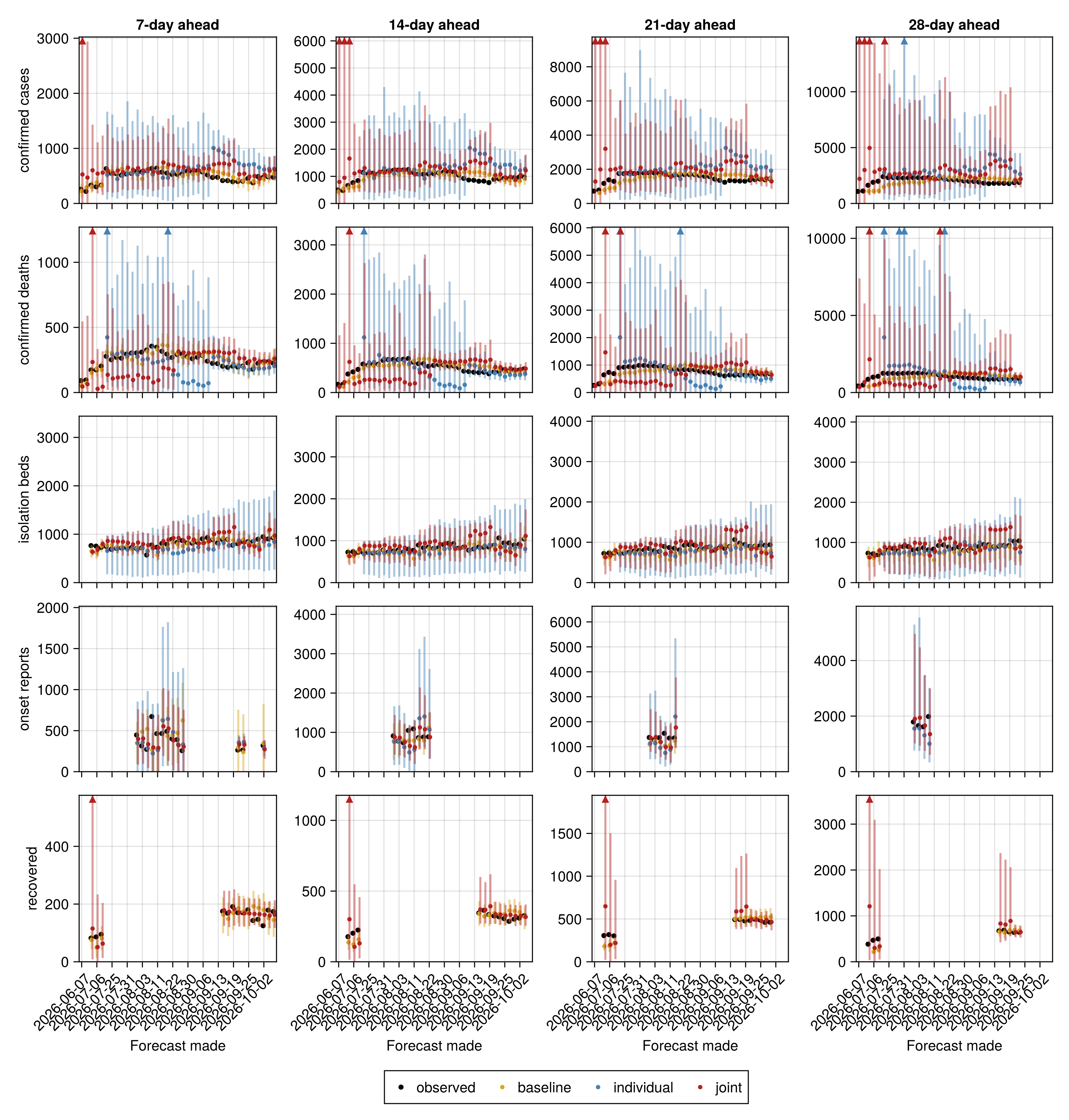
Forecasts-versus-now overlay
forecast_overlay_fig = plot_forecast_overlay(
    scored_overlay(forecast_overlay_df)
);
Frozen-fit forecast evaluation
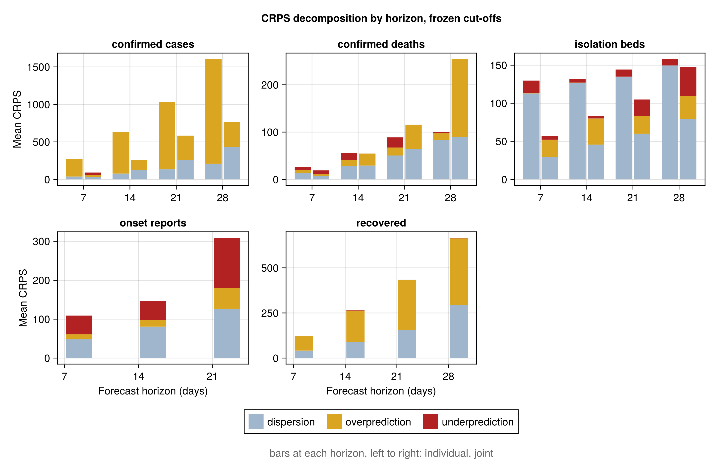
The current model, frozen at earlier data cut-offs (see forecast-versus-frozen evaluation), is scored as the cross-release forecasts above, against the same baseline. The tables in this section are the frozen joint model's, one row per stream. Each stream's own frozen fit is scored only at the one-week-back cut-off for still-reported streams, and appears in the skill figures rather than the tables. The May cut-offs predate the first reported bed occupancy and recoveries, so those windows are left unscored. The baseline snapshot was taken weeks after the frozen cut-off, so it can hold later revisions to earlier days (see forecast scoring against a persistence baseline).
Load and summarise the frozen-fit forecast scores
frozen_scores_df = _release_data(
    "forecast_scores_frozen.csv",
    (;
        release = String, made_date = Date, stream = String, horizon = Int,
        target_date = Date, fit = String, crps = Float64,
        log_crps = Float64, dispersion = Float64, overprediction = Float64,
        underprediction = Float64, coverage_50 = Float64,
        coverage_90 = Float64,
        bias = Float64, n_samples = Int,
        log_rel_to_baseline = Float64,
    )
)
frozen_overlay_df = _release_data(
    "forecast_overlay_frozen.csv",
    (;
        release = String, made_date = Date, stream = String, horizon = Int,
        target_date = Date, fit = String, observed = Float64,
        median = Float64, lo30 = Float64, hi30 = Float64, lo60 = Float64,
        hi60 = Float64, lo90 = Float64, hi90 = Float64,
    )
)
# Rows a superseded forecaster produced are dropped before anything is
# summarised or drawn, from the scores and the overlay alike, so the
# tables and the figures rest on one set of rows. See
# `drop_superseded_forecasts` for the one exclusion in force and why.
frozen_scores_df = _drop_rescanned(
    drop_superseded_forecasts(frozen_scores_df)
)
frozen_overlay_df = _drop_rescanned(
    drop_superseded_forecasts(frozen_overlay_df)
)

# The frozen joint carries `FROZEN_FIT`, so it is named as the joint role
# here and compared against each stream's own frozen fit. A release
# published before the archive had a `fit` column carries joint rows only.
frozen_score_overview_table = forecast_score_overview(
    frozen_scores_df; joint_fit = FROZEN_FIT
)
frozen_score_by_horizon_table = forecast_score_by_horizon(
    frozen_scores_df; joint_fit = FROZEN_FIT
)
frozen_score_by_release_table = forecast_score_by_release(
    frozen_scores_df; joint_fit = FROZEN_FIT
)

# The tables show the frozen joint alone, as the cross-release tables show
# the joint alone, so a row reads as one model at one cut-off rather than a
# stream interleaving two fits. The archive's single-stream frozen fits stay
# in the scored data and in the figures, which compare the roles against
# each other. Selecting the joint role leaves `fit` single-valued, so it is
# dropped and the model named in the prose instead.
_frozen_joint_only(tbl) = drop_degenerate_fit_column(
    select_fit_role(tbl, "joint")
)
frozen_score_overview_display = _frozen_joint_only(
    frozen_score_overview_table
)
frozen_score_by_horizon_display = _frozen_joint_only(
    frozen_score_by_horizon_table
)
frozen_score_by_release_display = _frozen_joint_only(
    frozen_score_by_release_table
)

# One row per release for the cut-offs more than one release forecast.
# See the comment above `joint_score_by_release_table`'s assignment for why
# this setup chunk's last statement needs a trailing `;`.
frozen_score_by_vintage_table = forecast_score_by_vintage(
    frozen_scores_df; joint_fit = FROZEN_FIT
)
frozen_score_by_vintage_display = _frozen_joint_only(
    frozen_score_by_vintage_table
);| stream | n | crps | rel_to_baseline | log_crps | log_rel_to_baseline | rel_to_individual | log_rel_to_individual | dispersion | overprediction | underprediction | coverage_50 | coverage_90 | bias |
|---|---|---|---|---|---|---|---|---|---|---|---|---|---|
| confirmed cases | 308 | 305.14 | 2.39 | 0.355 | 1.16 | 0.52 | 0.57 | 143.92 | 145.23 | 15.99 | 0.36 | 0.77 | 0.31 |
| confirmed deaths | 252 | 63.4 | 1.02 | 0.337 | 0.57 | 2.39 | 1.92 | 29.7 | 29.52 | 4.18 | 0.51 | 0.83 | 0.06 |
| isolation beds | 273 | 97.41 | 0.87 | 0.144 | 0.62 | 0.79 | 0.66 | 53.1 | 27.75 | 16.56 | 0.53 | 0.98 | 0.12 |
| onset reports | 30 | 148.16 | 1.03 | 0.245 | 0.84 | 69.53 | 19.73 | 58.91 | 0.57 | 0.9 | -0.16 | ||
| recovered | 133 | 363.06 | 7.77 | 0.584 | 4.49 | 140.76 | 220.05 | 2.25 | 0.42 | 0.62 | 0.53 |
frozen_relative_skill_fig = plot_forecast_relative_skill(
    frozen_score_by_horizon_table
);
frozen_crps_by_horizon_fig = plot_forecast_crps_by_horizon(
    frozen_score_by_horizon_table;
    title = "CRPS decomposition by horizon, frozen cut-offs"
);
Scores by horizon
| stream | horizon | n | crps | rel_to_baseline | log_crps | log_rel_to_baseline | rel_to_individual | log_rel_to_individual | dispersion | overprediction | underprediction | coverage_50 | coverage_90 | bias |
|---|---|---|---|---|---|---|---|---|---|---|---|---|---|---|
| confirmed cases | 7 | 140 | 91.15 | 1.07 | 0.391 | 0.77 | 0.49 | 0.55 | 32.95 | 23.02 | 35.18 | 0.38 | 0.71 | -0.07 |
| confirmed cases | 14 | 69 | 258.75 | 3.28 | 0.28 | 2.94 | 0.52 | 0.58 | 127.29 | 131.46 | 0 | 0.41 | 0.86 | 0.6 |
| confirmed cases | 21 | 68 | 583.22 | 3.67 | 0.398 | 2.57 | 0.53 | 0.58 | 257.57 | 325.65 | 0 | 0.22 | 0.74 | 0.69 |
| confirmed cases | 28 | 31 | 764.79 | 2.12 | 0.264 | 1.44 | 0.53 | 0.57 | 432.79 | 332 | 0 | 0.52 | 0.9 | 0.54 |
| confirmed deaths | 7 | 126 | 19.13 | 0.78 | 0.47 | 0.58 | 1.7 | 1.57 | 7.13 | 3.65 | 8.34 | 0.5 | 0.81 | -0.34 |
| confirmed deaths | 14 | 55 | 54.61 | 1.17 | 0.178 | 0.75 | 2.02 | 1.8 | 29.22 | 25.35 | 0.04 | 0.73 | 0.89 | 0.37 |
| confirmed deaths | 21 | 54 | 115.58 | 0.88 | 0.224 | 0.41 | 2.19 | 1.88 | 64.19 | 51.38 | 0.02 | 0.46 | 0.89 | 0.45 |
| confirmed deaths | 28 | 17 | 254.25 | 1.46 | 0.22 | 1.31 | 3.17 | 2.79 | 89.02 | 165.23 | 0 | 0.06 | 0.65 | 0.76 |
| isolation beds | 7 | 70 | 57.07 | 1.22 | 0.091 | 0.88 | 0.54 | 0.46 | 29.38 | 22.72 | 4.97 | 0.64 | 0.93 | 0.26 |
| isolation beds | 14 | 69 | 83.31 | 1.57 | 0.133 | 1.14 | 0.81 | 0.7 | 45.68 | 34.31 | 3.32 | 0.64 | 1 | 0.33 |
| isolation beds | 21 | 68 | 104.88 | 0.67 | 0.154 | 0.48 | 0.89 | 0.74 | 59.99 | 23.69 | 21.2 | 0.46 | 1 | -0.05 |
| isolation beds | 28 | 66 | 147.25 | 0.75 | 0.201 | 0.52 | 0.97 | 0.78 | 78.92 | 30.4 | 37.92 | 0.38 | 1 | -0.09 |
| onset reports | 7 | 16 | 109.12 | 0.75 | 0.293 | 0.7 | 48.18 | 12.92 | 48.02 | 0.56 | 0.88 | -0.2 | ||
| onset reports | 14 | 10 | 146.28 | 1.35 | 0.173 | 1.28 | 80.8 | 17.38 | 48.1 | 0.7 | 0.9 | -0.07 | ||
| onset reports | 21 | 4 | 309.05 | 1.36 | 0.238 | 1.31 | 126.71 | 52.85 | 129.49 | 0.25 | 1 | -0.27 | ||
| recovered | 7 | 35 | 122.59 | 6.45 | 0.546 | 4.25 | 41.66 | 79.5 | 1.42 | 0.4 | 0.83 | 0.5 | ||
| recovered | 14 | 34 | 264.8 | 10.59 | 0.569 | 6.46 | 88.35 | 174.54 | 1.9 | 0.41 | 0.56 | 0.54 | ||
| recovered | 21 | 33 | 434.07 | 7.69 | 0.601 | 4.4 | 155.08 | 276.55 | 2.44 | 0.42 | 0.55 | 0.54 | ||
| recovered | 28 | 31 | 666.75 | 7.28 | 0.624 | 3.64 | 294.89 | 368.48 | 3.37 | 0.45 | 0.52 | 0.52 |
frozen_skill_by_cutoff_fig = plot_forecast_skill_by_cutoff(
    frozen_score_by_release_table;
    xlabel = "Frozen cut-off",
    title = "Relative skill against the baseline, by frozen cut-off"
);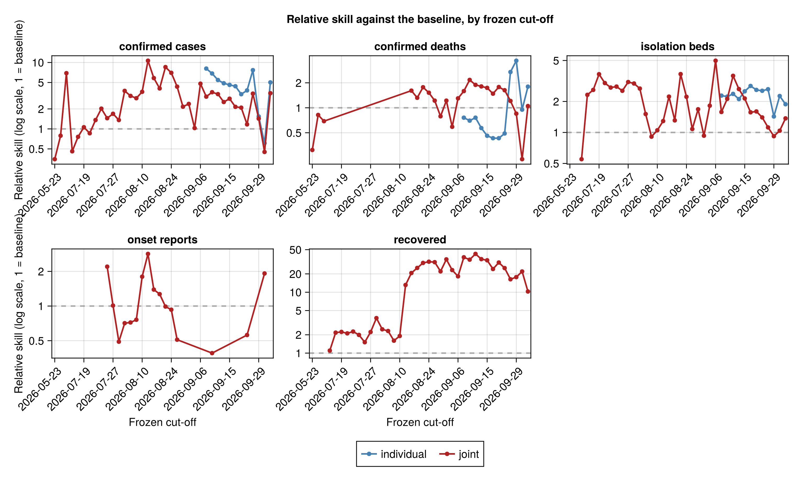
Scores by frozen cut-off
| made_date | stream | n | crps | rel_to_baseline | log_crps | log_rel_to_baseline | rel_to_individual | log_rel_to_individual | dispersion | overprediction | underprediction | coverage_50 | coverage_90 | bias |
|---|---|---|---|---|---|---|---|---|---|---|---|---|---|---|
| 2026-05-23 | confirmed cases | 35 | 29.37 | 0.35 | 0.192 | 0.31 | 18.61 | 0 | 10.75 | 0.6 | 1 | -0.37 | ||
| 2026-05-27 | confirmed cases | 35 | 141.53 | 0.79 | 0.936 | 0.75 | 11.91 | 0 | 129.63 | 0 | 0.09 | -0.95 | ||
| 2026-06-08 | confirmed cases | 105 | 342.3 | 6.91 | 0.381 | 3.97 | 147.8 | 194.5 | 0 | 0.25 | 0.85 | 0.67 | ||
| 2026-07-16 | confirmed cases | 4 | 294.68 | 0.46 | 0.168 | 0.29 | 283.46 | 10.98 | 0.24 | 1 | 1 | 0.07 | ||
| 2026-07-18 | confirmed cases | 4 | 361.26 | 0.76 | 0.185 | 0.5 | 333.85 | 27.41 | 0 | 1 | 1 | 0.15 | ||
| 2026-07-19 | confirmed cases | 4 | 439.62 | 1.06 | 0.209 | 0.7 | 351.83 | 87.79 | 0 | 1 | 1 | 0.3 | ||
| 2026-07-20 | confirmed cases | 4 | 385.62 | 0.86 | 0.185 | 0.55 | 332.6 | 53.02 | 0 | 1 | 1 | 0.22 | ||
| 2026-07-24 | confirmed cases | 4 | 422.92 | 1.36 | 0.192 | 0.95 | 343.7 | 79.22 | 0 | 1 | 1 | 0.32 | ||
| 2026-07-25 | confirmed cases | 4 | 460.72 | 2.02 | 0.209 | 1.52 | 356.82 | 103.91 | 0 | 1 | 1 | 0.34 | ||
| 2026-07-26 | confirmed cases | 4 | 315.56 | 1.45 | 0.164 | 1.27 | 284.59 | 30.97 | 0 | 1 | 1 | 0.24 | ||
| 2026-07-27 | confirmed cases | 4 | 346.39 | 1.69 | 0.176 | 1.29 | 306.97 | 39.42 | 0 | 1 | 1 | 0.27 | ||
| 2026-07-28 | confirmed cases | 4 | 396.78 | 1.36 | 0.156 | 0.84 | 361.52 | 35.26 | 0 | 1 | 1 | 0.22 | ||
| 2026-07-31 | confirmed cases | 4 | 498.38 | 3.74 | 0.213 | 2.49 | 369.58 | 128.8 | 0 | 0.75 | 1 | 0.38 | ||
| 2026-08-04 | confirmed cases | 4 | 281.57 | 3.14 | 0.156 | 2.89 | 253.99 | 27.59 | 0 | 1 | 1 | 0.18 | ||
| 2026-08-08 | confirmed cases | 4 | 253.51 | 2.9 | 0.15 | 2.14 | 246.67 | 6.12 | 0.72 | 1 | 1 | 0.03 | ||
| 2026-08-10 | confirmed cases | 4 | 244.51 | 3.62 | 0.15 | 2.56 | 241 | 1.7 | 1.81 | 1 | 1 | -0.01 | ||
| 2026-08-15 | confirmed cases | 4 | 623.4 | 10.65 | 0.281 | 5.59 | 384.1 | 239.3 | 0 | 0.25 | 1 | 0.52 | ||
| 2026-08-17 | confirmed cases | 4 | 426.55 | 5.83 | 0.234 | 3.63 | 166.54 | 260.01 | 0 | 0 | 1 | 0.75 | ||
| 2026-08-18 | confirmed cases | 4 | 468.25 | 4.07 | 0.276 | 2.88 | 155.86 | 312.4 | 0 | 0 | 0.75 | 0.85 | ||
| 2026-08-23 | confirmed cases | 4 | 562.74 | 8.53 | 0.314 | 6.6 | 140.78 | 421.96 | 0 | 0 | 0.75 | 0.88 | ||
| 2026-08-24 | confirmed cases | 4 | 437.04 | 6.99 | 0.246 | 5.65 | 160.51 | 276.53 | 0 | 0 | 0.75 | 0.82 | ||
| 2026-08-25 | confirmed cases | 4 | 288.32 | 4.33 | 0.176 | 3.96 | 113.18 | 175.14 | 0 | 0 | 1 | 0.74 | ||
| 2026-08-30 | confirmed cases | 4 | 179.54 | 2.16 | 0.106 | 1.68 | 110.05 | 69.49 | 0 | 0.75 | 1 | 0.44 | ||
| 2026-09-03 | confirmed cases | 4 | 279.85 | 2.38 | 0.161 | 2.28 | 99.17 | 180.68 | 0 | 0 | 1 | 0.71 | ||
| 2026-09-05 | confirmed cases | 4 | 133.12 | 1.03 | 0.084 | 1.02 | 104.06 | 28.72 | 0.34 | 1 | 1 | 0.19 | ||
| 2026-09-06 | confirmed cases | 4 | 560.62 | 4.8 | 0.279 | 3.83 | 181.89 | 378.73 | 0 | 0 | 1 | 0.74 | ||
| 2026-09-08 | confirmed cases | 4 | 439.23 | 3.06 | 0.241 | 2.46 | 0.38 | 0.39 | 185.89 | 253.34 | 0 | 0 | 0.75 | 0.76 |
| 2026-09-09 | confirmed cases | 4 | 610.51 | 3.57 | 0.331 | 2.75 | 0.52 | 0.52 | 205.84 | 404.67 | 0 | 0 | 0.5 | 0.85 |
| 2026-09-12 | confirmed cases | 4 | 810.13 | 3.34 | 0.484 | 2.54 | 0.61 | 0.64 | 191.69 | 618.44 | 0 | 0 | 0 | 0.96 |
| 2026-09-14 | confirmed cases | 4 | 591.66 | 2.54 | 0.417 | 2.03 | 0.52 | 0.6 | 111.41 | 480.25 | 0 | 0 | 0 | 0.97 |
| 2026-09-15 | confirmed cases | 4 | 641.05 | 2.85 | 0.45 | 2.27 | 0.62 | 0.68 | 126.77 | 514.28 | 0 | 0 | 0 | 0.97 |
| 2026-09-18 | confirmed cases | 4 | 433.84 | 2.15 | 0.353 | 1.95 | 0.49 | 0.58 | 92.05 | 341.79 | 0 | 0 | 0.25 | 0.95 |
| 2026-09-19 | confirmed cases | 4 | 410.13 | 2.09 | 0.325 | 1.97 | 0.63 | 0.67 | 117.34 | 292.79 | 0 | 0 | 0.5 | 0.88 |
| 2026-09-20 | confirmed cases | 4 | 175.25 | 1.17 | 0.163 | 1.3 | 0.31 | 0.38 | 86.67 | 88.58 | 0 | 0.25 | 0.75 | 0.67 |
| 2026-09-25 | confirmed cases | 3 | 145.31 | 3.4 | 0.138 | 2.21 | 0.44 | 0.47 | 60.17 | 85.14 | 0 | 0 | 1 | 0.71 |
| 2026-09-29 | confirmed cases | 3 | 111.26 | 1.43 | 0.091 | 0.87 | 0.93 | 0.83 | 74.48 | 36.78 | 0 | 1 | 1 | 0.4 |
| 2026-10-03 | confirmed cases | 2 | 66.82 | 0.45 | 0.074 | 0.32 | 0.73 | 0.72 | 52.46 | 14.36 | 0 | 1 | 1 | 0.28 |
| 2026-10-13 | confirmed cases | 1 | 64.31 | 3.45 | 0.115 | 2.96 | 0.69 | 0.7 | 29.09 | 35.22 | 0 | 0 | 1 | 0.67 |
| 2026-05-23 | confirmed deaths | 35 | 7.75 | 0.31 | 0.332 | 0.24 | 3.53 | 0 | 4.22 | 0.49 | 1 | -0.49 | ||
| 2026-05-27 | confirmed deaths | 35 | 26.55 | 0.82 | 1.099 | 0.92 | 2.24 | 0 | 24.31 | 0 | 0.49 | -0.91 | ||
| 2026-06-08 | confirmed deaths | 105 | 47.32 | 0.69 | 0.203 | 0.46 | 38.48 | 8.38 | 0.46 | 0.88 | 1 | 0.13 | ||
| 2026-08-17 | confirmed deaths | 4 | 91.87 | 1.61 | 0.097 | 1.14 | 59.3 | 32.57 | 0 | 0.5 | 1 | 0.44 | ||
| 2026-08-18 | confirmed deaths | 4 | 115.9 | 1.32 | 0.134 | 1.07 | 55.91 | 59.99 | 0 | 0 | 1 | 0.63 | ||
| 2026-08-23 | confirmed deaths | 4 | 145.19 | 1.77 | 0.166 | 1.56 | 51.71 | 93.48 | 0 | 0 | 1 | 0.72 | ||
| 2026-08-24 | confirmed deaths | 4 | 110.91 | 1.52 | 0.12 | 1.34 | 55.2 | 55.71 | 0 | 0.25 | 1 | 0.53 | ||
| 2026-08-25 | confirmed deaths | 4 | 87.42 | 1.22 | 0.1 | 1.18 | 44.65 | 42.77 | 0 | 0.25 | 1 | 0.53 | ||
| 2026-08-30 | confirmed deaths | 4 | 69.43 | 0.79 | 0.087 | 0.9 | 39.75 | 29.68 | 0 | 0.5 | 1 | 0.5 | ||
| 2026-09-03 | confirmed deaths | 4 | 94.77 | 1.22 | 0.112 | 1.18 | 41.4 | 53.37 | 0 | 0.25 | 1 | 0.55 | ||
| 2026-09-05 | confirmed deaths | 4 | 53.98 | 0.59 | 0.074 | 0.67 | 40.77 | 12.26 | 0.95 | 1 | 1 | 0.17 | ||
| 2026-09-06 | confirmed deaths | 4 | 122.5 | 1.3 | 0.142 | 1.26 | 45.32 | 76.87 | 0.31 | 0.5 | 1 | 0.46 | ||
| 2026-09-08 | confirmed deaths | 4 | 165.38 | 1.59 | 0.193 | 1.45 | 2.1 | 1.82 | 67.21 | 98.16 | 0 | 0.25 | 1 | 0.73 |
| 2026-09-09 | confirmed deaths | 4 | 216.82 | 2.17 | 0.252 | 1.83 | 3.1 | 2.52 | 78.5 | 138.31 | 0 | 0 | 1 | 0.79 |
| 2026-09-12 | confirmed deaths | 4 | 265.95 | 1.89 | 0.342 | 1.51 | 2.48 | 2.13 | 68.8 | 197.15 | 0 | 0 | 0 | 0.94 |
| 2026-09-14 | confirmed deaths | 4 | 216.78 | 1.81 | 0.317 | 1.62 | 3.16 | 2.8 | 28.06 | 188.72 | 0 | 0 | 0 | 0.99 |
| 2026-09-15 | confirmed deaths | 4 | 206.51 | 1.74 | 0.323 | 1.63 | 3.79 | 3.27 | 27.27 | 179.24 | 0 | 0 | 0 | 0.99 |
| 2026-09-18 | confirmed deaths | 4 | 157.26 | 1.48 | 0.289 | 1.51 | 3.45 | 2.99 | 23.78 | 133.48 | 0 | 0 | 0 | 0.98 |
| 2026-09-19 | confirmed deaths | 4 | 162.39 | 1.78 | 0.28 | 1.85 | 4.1 | 3.8 | 26.75 | 135.64 | 0 | 0 | 0 | 0.97 |
| 2026-09-20 | confirmed deaths | 4 | 118.96 | 1.63 | 0.219 | 1.87 | 3.35 | 3.19 | 21.71 | 97.25 | 0 | 0 | 0 | 0.96 |
| 2026-09-25 | confirmed deaths | 3 | 34.22 | 1.21 | 0.071 | 0.83 | 0.45 | 0.39 | 16.6 | 17.63 | 0 | 0 | 1 | 0.58 |
| 2026-09-29 | confirmed deaths | 3 | 19.36 | 0.85 | 0.045 | 0.8 | 0.23 | 0.23 | 17.14 | 1.94 | 0.29 | 1 | 1 | 0.14 |
| 2026-10-03 | confirmed deaths | 2 | 14.05 | 0.24 | 0.04 | 0.2 | 0.25 | 0.22 | 13.34 | 0.02 | 0.69 | 1 | 1 | -0.12 |
| 2026-10-13 | confirmed deaths | 1 | 11.3 | 1.05 | 0.044 | 0.96 | 0.58 | 0.51 | 10.76 | 0.54 | 0 | 1 | 1 | 0.13 |
| 2026-06-08 | isolation beds | 140 | 91.72 | 0.55 | 0.16 | 0.41 | 51.01 | 15.27 | 25.44 | 0.51 | 1 | -0.04 | ||
| 2026-07-16 | isolation beds | 4 | 73.22 | 2.32 | 0.096 | 2.2 | 20.01 | 53.22 | 0 | 0 | 1 | 0.6 | ||
| 2026-07-18 | isolation beds | 4 | 77.78 | 2.59 | 0.103 | 2.46 | 18.71 | 59.07 | 0 | 0 | 1 | 0.61 | ||
| 2026-07-19 | isolation beds | 4 | 100.01 | 3.68 | 0.132 | 3.53 | 22.38 | 77.63 | 0 | 0 | 1 | 0.64 | ||
| 2026-07-20 | isolation beds | 4 | 82.23 | 3.02 | 0.106 | 2.87 | 19.89 | 62.33 | 0 | 0.25 | 1 | 0.61 | ||
| 2026-07-24 | isolation beds | 4 | 76.61 | 2.73 | 0.096 | 2.56 | 10.14 | 66.47 | 0 | 0 | 1 | 0.73 | ||
| 2026-07-25 | isolation beds | 4 | 106.43 | 2.79 | 0.136 | 2.69 | 13.84 | 92.59 | 0 | 0 | 0.75 | 0.73 | ||
| 2026-07-26 | isolation beds | 4 | 94.88 | 2.54 | 0.122 | 2.4 | 22.61 | 72.27 | 0 | 0.25 | 0.75 | 0.63 | ||
| 2026-07-27 | isolation beds | 4 | 85.56 | 3.09 | 0.113 | 2.99 | 38.92 | 46.65 | 0 | 0.5 | 1 | 0.48 | ||
| 2026-07-28 | isolation beds | 4 | 153.08 | 2.99 | 0.201 | 2.67 | 41.15 | 111.94 | 0 | 0.5 | 0.75 | 0.67 | ||
| 2026-07-31 | isolation beds | 4 | 119.06 | 2.67 | 0.139 | 2.43 | 41.36 | 77.7 | 0 | 0.5 | 0.75 | 0.57 | ||
| 2026-08-04 | isolation beds | 4 | 110.51 | 1.51 | 0.153 | 1.46 | 63.26 | 47.24 | 0 | 0.75 | 0.75 | 0.42 | ||
| 2026-08-08 | isolation beds | 4 | 59.17 | 0.91 | 0.078 | 0.92 | 51.54 | 7.15 | 0.48 | 0.75 | 1 | 0.16 | ||
| 2026-08-10 | isolation beds | 4 | 55.99 | 1.05 | 0.079 | 1.1 | 55.83 | 0.02 | 0.15 | 1 | 1 | 0 | ||
| 2026-08-15 | isolation beds | 4 | 109.36 | 1.29 | 0.115 | 1.08 | 74.07 | 35.3 | 0 | 1 | 1 | 0.34 | ||
| 2026-08-17 | isolation beds | 4 | 103.6 | 2.23 | 0.111 | 1.92 | 72.62 | 30.98 | 0 | 0.75 | 1 | 0.43 | ||
| 2026-08-18 | isolation beds | 4 | 93.5 | 1.31 | 0.1 | 1.09 | 71.31 | 22.19 | 0 | 0.75 | 1 | 0.34 | ||
| 2026-08-23 | isolation beds | 4 | 145.69 | 3.69 | 0.149 | 3.17 | 60.67 | 85.02 | 0 | 0 | 1 | 0.66 | ||
| 2026-08-24 | isolation beds | 4 | 108.37 | 2.22 | 0.113 | 1.89 | 68.47 | 39.9 | 0 | 0.5 | 1 | 0.46 | ||
| 2026-08-25 | isolation beds | 4 | 71.1 | 1.08 | 0.087 | 1.06 | 60.24 | 0 | 10.86 | 1 | 1 | -0.27 | ||
| 2026-08-30 | isolation beds | 4 | 71.87 | 1.68 | 0.094 | 1.78 | 62.25 | 0 | 9.62 | 1 | 1 | -0.19 | ||
| 2026-09-03 | isolation beds | 4 | 76.35 | 0.93 | 0.096 | 0.92 | 53.15 | 0 | 23.2 | 0.75 | 1 | -0.38 | ||
| 2026-09-05 | isolation beds | 4 | 86.59 | 1.82 | 0.112 | 2.01 | 67.81 | 0 | 18.78 | 0.75 | 1 | -0.31 | ||
| 2026-09-06 | isolation beds | 4 | 243.91 | 4.98 | 0.522 | 8.74 | 146.37 | 0 | 97.55 | 0.75 | 1 | -0.44 | ||
| 2026-09-08 | isolation beds | 4 | 106.03 | 1.58 | 0.108 | 1.42 | 0.7 | 0.53 | 91.12 | 14.14 | 0.76 | 1 | 1 | 0.12 |
| 2026-09-09 | isolation beds | 4 | 136.55 | 2.12 | 0.132 | 1.71 | 0.95 | 0.66 | 81.86 | 54.69 | 0 | 0.75 | 1 | 0.37 |
| 2026-09-12 | isolation beds | 4 | 198.78 | 3.55 | 0.196 | 3.11 | 1.5 | 1.16 | 49.76 | 149.02 | 0 | 0 | 1 | 0.7 |
| 2026-09-14 | isolation beds | 4 | 164.32 | 2.64 | 0.159 | 2.32 | 1.25 | 1.01 | 75.68 | 88.64 | 0 | 0 | 1 | 0.7 |
| 2026-09-15 | isolation beds | 4 | 115.22 | 2.14 | 0.11 | 1.91 | 0.85 | 0.68 | 75.23 | 40 | 0 | 0.5 | 1 | 0.43 |
| 2026-09-18 | isolation beds | 4 | 74.76 | 1.57 | 0.078 | 1.45 | 0.55 | 0.47 | 62.67 | 12.09 | 0 | 0.75 | 1 | 0.27 |
| 2026-09-19 | isolation beds | 4 | 84.48 | 1.6 | 0.089 | 1.46 | 0.62 | 0.56 | 71.26 | 13.2 | 0.02 | 0.75 | 1 | 0.24 |
| 2026-09-20 | isolation beds | 4 | 78.16 | 1.4 | 0.097 | 1.44 | 0.55 | 0.57 | 59.17 | 0 | 19 | 1 | 1 | -0.32 |
| 2026-09-25 | isolation beds | 3 | 57.24 | 1.12 | 0.066 | 1.09 | 0.43 | 0.43 | 48 | 0 | 9.24 | 1 | 1 | -0.19 |
| 2026-09-29 | isolation beds | 3 | 99.08 | 0.92 | 0.107 | 0.93 | 0.64 | 0.58 | 57.97 | 0 | 41.12 | 0.67 | 1 | -0.4 |
| 2026-10-03 | isolation beds | 2 | 59.46 | 1.04 | 0.065 | 0.98 | 0.46 | 0.41 | 55.25 | 0 | 4.22 | 1 | 1 | -0.12 |
| 2026-10-13 | isolation beds | 1 | 111.96 | 1.37 | 0.119 | 1.41 | 0.73 | 0.68 | 33 | 0 | 78.96 | 0 | 1 | -0.76 |
| 2026-07-26 | onset reports | 2 | 67.83 | 2.2 | 0.119 | 1.98 | 65.22 | 2.61 | 0 | 1 | 1 | 0.13 | ||
| 2026-07-27 | onset reports | 2 | 68.12 | 1.01 | 0.121 | 0.81 | 56.66 | 1.46 | 10.01 | 1 | 1 | -0.15 | ||
| 2026-07-28 | onset reports | 2 | 79 | 0.49 | 0.129 | 0.37 | 61.39 | 6.94 | 10.67 | 1 | 1 | -0.07 | ||
| 2026-07-31 | onset reports | 2 | 117.29 | 0.71 | 0.239 | 0.61 | 75.72 | 41.58 | 0 | 0.5 | 1 | 0.4 | ||
| 2026-08-04 | onset reports | 3 | 94 | 0.72 | 0.137 | 0.62 | 67.9 | 1.45 | 24.65 | 1 | 1 | -0.14 | ||
| 2026-08-08 | onset reports | 3 | 341.25 | 0.76 | 0.477 | 0.71 | 71.38 | 0 | 269.88 | 0 | 0.33 | -0.88 | ||
| 2026-08-10 | onset reports | 3 | 198.52 | 1.8 | 0.309 | 1.92 | 66.1 | 0 | 132.41 | 0 | 1 | -0.69 | ||
| 2026-08-15 | onset reports | 3 | 263.97 | 2.84 | 0.215 | 1.78 | 135.96 | 128.01 | 0 | 0.33 | 1 | 0.64 | ||
| 2026-08-17 | onset reports | 2 | 83.46 | 1.39 | 0.178 | 1.67 | 71.82 | 0 | 11.64 | 1 | 1 | -0.25 | ||
| 2026-08-18 | onset reports | 2 | 114.86 | 1.27 | 0.24 | 1.55 | 78.01 | 0 | 36.85 | 0.5 | 1 | -0.33 | ||
| 2026-08-23 | onset reports | 1 | 64.41 | 0.99 | 0.222 | 1.31 | 58.23 | 0 | 6.18 | 1 | 1 | -0.2 | ||
| 2026-08-24 | onset reports | 1 | 70.4 | 0.93 | 0.322 | 1.84 | 62.25 | 0 | 8.15 | 1 | 1 | -0.21 | ||
| 2026-08-25 | onset reports | 1 | 124.18 | 0.51 | 0.36 | 0.6 | 35.28 | 88.9 | 0 | 0 | 1 | 0.81 | ||
| 2026-09-09 | onset reports | 1 | 67.92 | 0.39 | 0.124 | 0.15 | 58.46 | 9.46 | 0 | 1 | 1 | 0.23 | ||
| 2026-09-20 | onset reports | 1 | 56.91 | 0.56 | 0.166 | 0.26 | 14.2 | 0 | 42.7 | 0 | 1 | -0.8 | ||
| 2026-10-03 | onset reports | 1 | 306.69 | 1.92 | 0.698 | 1.73 | 15.69 | 0 | 291 | 0 | 0 | -1 | ||
| 2026-07-16 | recovered | 4 | 139.34 | 1.1 | 0.469 | 1.11 | 135.5 | 0 | 3.84 | 1 | 1 | -0.1 | ||
| 2026-07-18 | recovered | 4 | 149.61 | 2.17 | 0.455 | 2.13 | 146.94 | 2.67 | 0 | 1 | 1 | 0.1 | ||
| 2026-07-19 | recovered | 4 | 181.47 | 2.23 | 0.482 | 2.12 | 179.35 | 2.12 | 0 | 1 | 1 | 0.07 | ||
| 2026-07-20 | recovered | 4 | 171.81 | 2.11 | 0.417 | 1.91 | 169.63 | 2.18 | 0 | 1 | 1 | 0.06 | ||
| 2026-07-24 | recovered | 4 | 179.37 | 2.26 | 0.409 | 1.95 | 175.36 | 4.01 | 0 | 1 | 1 | 0.13 | ||
| 2026-07-25 | recovered | 4 | 177.7 | 1.99 | 0.379 | 1.66 | 173.52 | 4.18 | 0 | 1 | 1 | 0.12 | ||
| 2026-07-26 | recovered | 4 | 139.99 | 1.51 | 0.381 | 1.59 | 138.99 | 0 | 1 | 1 | 1 | -0.05 | ||
| 2026-07-27 | recovered | 4 | 219.87 | 2.22 | 0.483 | 1.86 | 218.38 | 0 | 1.49 | 1 | 1 | -0.06 | ||
| 2026-07-28 | recovered | 4 | 544.07 | 3.76 | 0.369 | 0.85 | 543.25 | 0.5 | 0.33 | 1 | 1 | 0.02 | ||
| 2026-07-31 | recovered | 4 | 249.16 | 2.46 | 0.402 | 1.48 | 242.91 | 6.25 | 0 | 1 | 1 | 0.12 | ||
| 2026-08-04 | recovered | 4 | 157.98 | 2.31 | 0.457 | 2.65 | 146.41 | 0 | 11.57 | 1 | 1 | -0.19 | ||
| 2026-08-08 | recovered | 4 | 125.59 | 1.6 | 0.417 | 2.09 | 109.72 | 0 | 15.87 | 1 | 1 | -0.23 | ||
| 2026-08-10 | recovered | 4 | 157.1 | 1.91 | 0.537 | 2.47 | 116.31 | 0 | 40.79 | 1 | 1 | -0.32 | ||
| 2026-08-15 | recovered | 4 | 384.45 | 13.15 | 0.442 | 5.97 | 335.62 | 48.83 | 0 | 1 | 1 | 0.29 | ||
| 2026-08-17 | recovered | 4 | 548.58 | 20.68 | 0.779 | 9.23 | 117.93 | 430.64 | 0 | 0 | 0 | 0.94 | ||
| 2026-08-18 | recovered | 4 | 596.27 | 25.05 | 0.834 | 11.62 | 99.02 | 497.25 | 0 | 0 | 0 | 0.95 | ||
| 2026-08-23 | recovered | 4 | 553.29 | 30.28 | 0.739 | 15.62 | 114.01 | 439.28 | 0 | 0 | 0.25 | 0.92 | ||
| 2026-08-24 | recovered | 4 | 518.58 | 31.72 | 0.726 | 16.52 | 112.37 | 406.22 | 0 | 0 | 0 | 0.94 | ||
| 2026-08-25 | recovered | 4 | 500.24 | 31.17 | 0.716 | 16.75 | 90.53 | 409.71 | 0 | 0 | 0 | 0.96 | ||
| 2026-08-30 | recovered | 4 | 436.88 | 22.01 | 0.635 | 12.74 | 97.38 | 339.5 | 0 | 0 | 0.25 | 0.92 | ||
| 2026-09-03 | recovered | 4 | 505.86 | 34.65 | 0.714 | 19.39 | 94.33 | 411.53 | 0 | 0 | 0.25 | 0.92 | ||
| 2026-09-05 | recovered | 4 | 369.4 | 23.1 | 0.582 | 13.29 | 88.66 | 280.73 | 0 | 0 | 0.5 | 0.89 | ||
| 2026-09-06 | recovered | 4 | 295.01 | 18.23 | 0.43 | 10.29 | 95.6 | 199.41 | 0 | 0 | 0.5 | 0.79 | ||
| 2026-09-08 | recovered | 4 | 563.28 | 37.49 | 0.75 | 19.76 | 133.12 | 430.16 | 0 | 0 | 0.5 | 0.9 | ||
| 2026-09-09 | recovered | 4 | 621.79 | 34.25 | 0.839 | 16.48 | 139.18 | 482.61 | 0 | 0 | 0 | 0.97 | ||
| 2026-09-12 | recovered | 4 | 633.36 | 42.62 | 0.794 | 20.81 | 139.51 | 493.85 | 0 | 0 | 0.25 | 0.94 | ||
| 2026-09-14 | recovered | 4 | 481.67 | 34.95 | 0.675 | 16.12 | 75.86 | 405.81 | 0 | 0 | 0 | 0.94 | ||
| 2026-09-15 | recovered | 4 | 487.5 | 33.47 | 0.683 | 17.38 | 87.32 | 400.18 | 0 | 0 | 0.5 | 0.91 | ||
| 2026-09-18 | recovered | 4 | 458.84 | 24.05 | 0.681 | 14.91 | 73.88 | 384.96 | 0 | 0 | 0.25 | 0.92 | ||
| 2026-09-19 | recovered | 4 | 518.14 | 30.74 | 0.728 | 15.45 | 84.46 | 433.69 | 0 | 0 | 0.25 | 0.93 | ||
| 2026-09-20 | recovered | 4 | 406.23 | 24.93 | 0.609 | 14.87 | 81.49 | 324.74 | 0 | 0 | 1 | 0.85 | ||
| 2026-09-25 | recovered | 3 | 273.4 | 16.32 | 0.543 | 10.46 | 61.12 | 212.28 | 0 | 0 | 1 | 0.82 | ||
| 2026-09-29 | recovered | 3 | 311.28 | 17.71 | 0.635 | 10.89 | 59.96 | 251.32 | 0 | 0 | 1 | 0.88 | ||
| 2026-10-03 | recovered | 2 | 223.85 | 21.91 | 0.636 | 14.03 | 47.81 | 176.04 | 0 | 0 | 0.5 | 0.89 | ||
| 2026-10-13 | recovered | 1 | 195.98 | 10.28 | 0.763 | 6.66 | 36.6 | 159.37 | 0 | 0 | 1 | 0.83 |
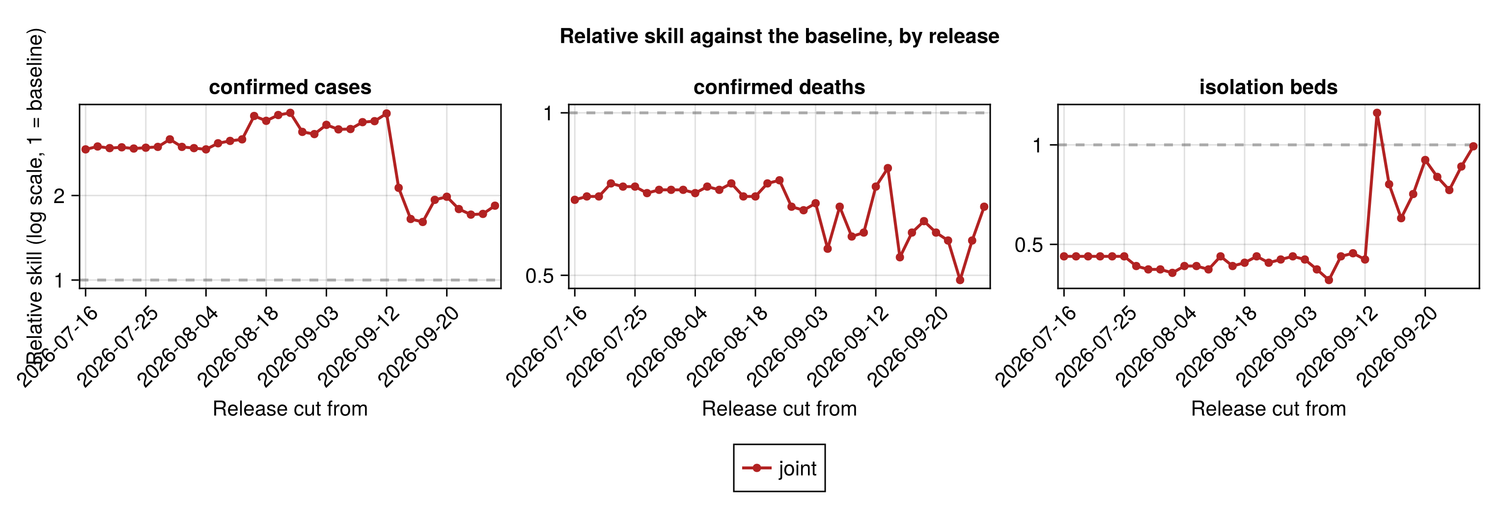
Frozen skill by release
Frozen skill per release
frozen_skill_by_vintage_fig = plot_forecast_skill_by_vintage(
    frozen_score_by_vintage_table
);
Frozen scores by release
| stream | release | release_date | n | crps | rel_to_baseline | log_crps | log_rel_to_baseline | rel_to_individual | log_rel_to_individual | dispersion | overprediction | underprediction | coverage_50 | coverage_90 | bias |
|---|---|---|---|---|---|---|---|---|---|---|---|---|---|---|---|
| confirmed cases | results-1359 | 2026-07-16 | 5 | 242.1 | 2.92 | 0.454 | 1.04 | 121.44 | 95.46 | 25.2 | 0.6 | 1 | 0.07 | ||
| confirmed cases | results-1391 | 2026-07-18 | 5 | 242.1 | 2.99 | 0.454 | 1.07 | 121.44 | 95.46 | 25.2 | 0.6 | 1 | 0.07 | ||
| confirmed cases | results-1394 | 2026-07-19 | 5 | 242.1 | 2.95 | 0.454 | 1.07 | 121.44 | 95.46 | 25.2 | 0.6 | 1 | 0.07 | ||
| confirmed cases | results-1441 | 2026-07-20 | 5 | 245.99 | 2.97 | 0.466 | 1.07 | 113.62 | 106.92 | 25.45 | 0.2 | 0.8 | 0.16 | ||
| confirmed cases | results-1446 | 2026-07-24 | 5 | 245.99 | 2.94 | 0.466 | 1.08 | 113.62 | 106.92 | 25.45 | 0.2 | 0.8 | 0.16 | ||
| confirmed cases | results-v1.12.0 | 2026-07-25 | 5 | 245.99 | 2.96 | 0.466 | 1.09 | 113.62 | 106.92 | 25.45 | 0.2 | 0.8 | 0.16 | ||
| confirmed cases | results-1462 | 2026-07-26 | 5 | 247.61 | 2.98 | 0.458 | 1.06 | 122.27 | 99.46 | 25.89 | 0.6 | 0.8 | 0.13 | ||
| confirmed cases | results-1469 | 2026-07-27 | 5 | 247.61 | 3.17 | 0.458 | 1.08 | 122.27 | 99.46 | 25.89 | 0.6 | 0.8 | 0.13 | ||
| confirmed cases | results-1479 | 2026-07-28 | 5 | 247.61 | 2.98 | 0.458 | 1.07 | 122.27 | 99.46 | 25.89 | 0.6 | 0.8 | 0.13 | ||
| confirmed cases | results-1489 | 2026-07-31 | 5 | 247.61 | 2.95 | 0.458 | 1.06 | 122.27 | 99.46 | 25.89 | 0.6 | 0.8 | 0.13 | ||
| confirmed cases | results-v1.13.2 | 2026-08-04 | 5 | 247.61 | 2.92 | 0.458 | 1.05 | 122.27 | 99.46 | 25.89 | 0.6 | 0.8 | 0.13 | ||
| confirmed cases | results-1505 | 2026-08-08 | 5 | 247.61 | 3.07 | 0.458 | 1.08 | 122.27 | 99.46 | 25.89 | 0.6 | 0.8 | 0.13 | ||
| confirmed cases | results-1527 | 2026-08-10 | 5 | 247.61 | 3.13 | 0.458 | 1.1 | 122.27 | 99.46 | 25.89 | 0.6 | 0.8 | 0.13 | ||
| confirmed cases | results-1573 | 2026-08-15 | 5 | 256.51 | 3.17 | 0.471 | 1.1 | 131.58 | 99.04 | 25.89 | 0.4 | 0.8 | 0.13 | ||
| confirmed cases | results-1591 | 2026-08-17 | 5 | 304.06 | 3.84 | 0.509 | 1.2 | 85.78 | 190.69 | 27.59 | 0.2 | 0.6 | 0.3 | ||
| confirmed cases | results-v1.15.0 | 2026-08-18 | 5 | 304.06 | 3.69 | 0.509 | 1.16 | 85.78 | 190.69 | 27.59 | 0.2 | 0.6 | 0.3 | ||
| confirmed cases | results-v1.16.0 | 2026-08-23 | 5 | 318.57 | 3.87 | 0.513 | 1.19 | 95.65 | 195.73 | 27.19 | 0.2 | 0.4 | 0.3 | ||
| confirmed cases | results-1625 | 2026-08-24 | 5 | 318.42 | 3.94 | 0.513 | 1.21 | 95.56 | 195.73 | 27.13 | 0.2 | 0.4 | 0.3 | ||
| confirmed cases | results-v1.17.0 | 2026-08-25 | 5 | 278.34 | 3.37 | 0.471 | 1.09 | 82.69 | 170.13 | 25.51 | 0.2 | 0.4 | 0.28 | ||
| confirmed cases | results-v1.18.0 | 2026-08-30 | 5 | 278.34 | 3.31 | 0.471 | 1.08 | 82.69 | 170.13 | 25.51 | 0.2 | 0.4 | 0.28 | ||
| confirmed cases | results-1739 | 2026-09-03 | 5 | 288.7 | 3.57 | 0.475 | 1.11 | 92.73 | 169.11 | 26.86 | 0.2 | 0.6 | 0.22 | ||
| confirmed cases | results-1828 | 2026-09-05 | 5 | 285.09 | 3.44 | 0.505 | 1.17 | 102.17 | 151.58 | 31.35 | 0 | 0.6 | 0.15 | ||
| confirmed cases | results-1858 | 2026-09-06 | 5 | 290.99 | 3.45 | 0.509 | 1.19 | 88.02 | 171.62 | 31.35 | 0 | 0.6 | 0.14 | ||
| confirmed cases | results-1970 | 2026-09-08 | 5 | 295.58 | 3.65 | 0.518 | 1.23 | 96.92 | 166.9 | 31.77 | 0 | 0.6 | 0.15 | ||
| confirmed cases | results-v2.1.0 | 2026-09-09 | 5 | 295.58 | 3.68 | 0.518 | 1.21 | 96.92 | 166.9 | 31.77 | 0 | 0.6 | 0.15 | ||
| confirmed cases | results-2177 | 2026-09-12 | 5 | 311.38 | 3.92 | 0.501 | 1.18 | 106.74 | 175.69 | 28.95 | 0 | 0.6 | 0.19 | ||
| confirmed cases | results-2360 | 2026-09-14 | 5 | 174.79 | 2.13 | 0.422 | 0.98 | 66.84 | 74.44 | 33.51 | 0 | 0.8 | 0.07 | ||
| confirmed cases | results-2506 | 2026-09-15 | 5 | 140.97 | 1.65 | 0.362 | 0.82 | 58.18 | 53.18 | 29.61 | 0.2 | 0.8 | 0.02 | ||
| confirmed cases | results-2536 | 2026-09-18 | 5 | 135.09 | 1.61 | 0.366 | 0.85 | 48.92 | 55.08 | 31.09 | 0.2 | 0.8 | 0.03 | ||
| confirmed cases | results-2720 | 2026-09-19 | 5 | 161.24 | 1.93 | 0.399 | 0.92 | 56.22 | 73.12 | 31.89 | 0 | 0.8 | 0.08 | ||
| confirmed cases | results-v3.0.0 | 2026-09-20 | 5 | 162.59 | 1.98 | 0.398 | 0.92 | 56.96 | 74.23 | 31.4 | 0 | 0.8 | 0.1 | ||
| confirmed cases | results-2968 | 2026-09-25 | 5 | 151.78 | 1.79 | 0.396 | 0.91 | 55.65 | 63.72 | 32.41 | 0.2 | 0.8 | 0.03 | ||
| confirmed cases | results-3000 | 2026-09-29 | 5 | 142.69 | 1.71 | 0.379 | 0.87 | 56.14 | 55.42 | 31.12 | 0 | 0.8 | 0.06 | ||
| confirmed cases | results-3086 | 2026-10-03 | 5 | 141.83 | 1.72 | 0.366 | 0.86 | 56.66 | 54.51 | 30.66 | 0.2 | 0.8 | 0.03 | ||
| confirmed cases | results-3140 | 2026-10-13 | 5 | 150.45 | 1.84 | 0.371 | 0.87 | 57.53 | 63.63 | 29.29 | 0.2 | 0.8 | 0.04 | ||
| confirmed deaths | results-1359 | 2026-07-16 | 5 | 36.61 | 0.69 | 0.553 | 0.7 | 28.04 | 0.07 | 8.49 | 0.6 | 0.8 | -0.39 | ||
| confirmed deaths | results-1391 | 2026-07-18 | 5 | 36.61 | 0.7 | 0.553 | 0.71 | 28.04 | 0.07 | 8.49 | 0.6 | 0.8 | -0.39 | ||
| confirmed deaths | results-1394 | 2026-07-19 | 5 | 36.61 | 0.7 | 0.553 | 0.69 | 28.04 | 0.07 | 8.49 | 0.6 | 0.8 | -0.39 | ||
| confirmed deaths | results-1441 | 2026-07-20 | 5 | 37.95 | 0.74 | 0.579 | 0.74 | 28.76 | 0.44 | 8.76 | 0.6 | 0.8 | -0.35 | ||
| confirmed deaths | results-1446 | 2026-07-24 | 5 | 37.95 | 0.73 | 0.579 | 0.74 | 28.76 | 0.44 | 8.76 | 0.6 | 0.8 | -0.35 | ||
| confirmed deaths | results-v1.12.0 | 2026-07-25 | 5 | 37.95 | 0.73 | 0.579 | 0.74 | 28.76 | 0.44 | 8.76 | 0.6 | 0.8 | -0.35 | ||
| confirmed deaths | results-1462 | 2026-07-26 | 5 | 37.32 | 0.71 | 0.635 | 0.8 | 27.48 | 0 | 9.84 | 0.6 | 0.8 | -0.43 | ||
| confirmed deaths | results-1469 | 2026-07-27 | 5 | 37.32 | 0.72 | 0.635 | 0.8 | 27.48 | 0 | 9.84 | 0.6 | 0.8 | -0.43 | ||
| confirmed deaths | results-1479 | 2026-07-28 | 5 | 37.32 | 0.72 | 0.635 | 0.81 | 27.48 | 0 | 9.84 | 0.6 | 0.8 | -0.43 | ||
| confirmed deaths | results-1489 | 2026-07-31 | 5 | 37.32 | 0.72 | 0.635 | 0.8 | 27.48 | 0 | 9.84 | 0.6 | 0.8 | -0.43 | ||
| confirmed deaths | results-v1.13.2 | 2026-08-04 | 5 | 37.32 | 0.71 | 0.635 | 0.8 | 27.48 | 0 | 9.84 | 0.6 | 0.8 | -0.43 | ||
| confirmed deaths | results-1505 | 2026-08-08 | 5 | 37.32 | 0.73 | 0.635 | 0.82 | 27.48 | 0 | 9.84 | 0.6 | 0.8 | -0.43 | ||
| confirmed deaths | results-1527 | 2026-08-10 | 5 | 37.32 | 0.72 | 0.635 | 0.82 | 27.48 | 0 | 9.84 | 0.6 | 0.8 | -0.43 | ||
| confirmed deaths | results-1573 | 2026-08-15 | 5 | 37.79 | 0.74 | 0.631 | 0.81 | 27.84 | 0.14 | 9.82 | 0.6 | 0.8 | -0.4 | ||
| confirmed deaths | results-1591 | 2026-08-17 | 5 | 36.94 | 0.7 | 0.288 | 0.36 | 20.9 | 12.14 | 3.9 | 0.6 | 1 | 0 | ||
| confirmed deaths | results-v1.15.0 | 2026-08-18 | 5 | 36.94 | 0.7 | 0.288 | 0.37 | 20.9 | 12.14 | 3.9 | 0.6 | 1 | 0 | ||
| confirmed deaths | results-v1.16.0 | 2026-08-23 | 5 | 38.99 | 0.74 | 0.27 | 0.35 | 24.17 | 11.59 | 3.22 | 0.6 | 1 | 0.04 | ||
| confirmed deaths | results-1625 | 2026-08-24 | 5 | 38.96 | 0.75 | 0.27 | 0.34 | 24.15 | 11.59 | 3.22 | 0.6 | 1 | 0.05 | ||
| confirmed deaths | results-v1.17.0 | 2026-08-25 | 5 | 35.05 | 0.67 | 0.256 | 0.33 | 21.96 | 10.14 | 2.94 | 0.6 | 1 | -0.03 | ||
| confirmed deaths | results-v1.18.0 | 2026-08-30 | 5 | 35.05 | 0.66 | 0.256 | 0.32 | 21.96 | 10.14 | 2.94 | 0.6 | 1 | -0.03 | ||
| confirmed deaths | results-1739 | 2026-09-03 | 5 | 34.71 | 0.68 | 0.274 | 0.35 | 22.91 | 8.35 | 3.45 | 0.6 | 1 | -0.02 | ||
| confirmed deaths | results-1828 | 2026-09-05 | 5 | 28.72 | 0.56 | 0.295 | 0.38 | 20.39 | 3.26 | 5.07 | 0.6 | 0.8 | -0.21 | ||
| confirmed deaths | results-1858 | 2026-09-06 | 5 | 35.33 | 0.67 | 0.314 | 0.4 | 21.97 | 8.26 | 5.1 | 0.6 | 0.8 | -0.17 | ||
| confirmed deaths | results-1970 | 2026-09-08 | 5 | 31.57 | 0.59 | 0.296 | 0.37 | 22.6 | 4.24 | 4.73 | 0.6 | 0.8 | -0.19 | ||
| confirmed deaths | results-v2.1.0 | 2026-09-09 | 5 | 31.57 | 0.6 | 0.296 | 0.38 | 22.6 | 4.24 | 4.73 | 0.6 | 0.8 | -0.19 | ||
| confirmed deaths | results-2177 | 2026-09-12 | 5 | 39.44 | 0.73 | 0.293 | 0.37 | 25.67 | 9.91 | 3.86 | 0.6 | 1 | -0.05 | ||
| confirmed deaths | results-2360 | 2026-09-14 | 5 | 41.87 | 0.79 | 0.294 | 0.37 | 23.54 | 14.65 | 3.68 | 0.4 | 1 | 0.01 | ||
| confirmed deaths | results-2506 | 2026-09-15 | 5 | 28.5 | 0.54 | 0.252 | 0.31 | 20.71 | 4.24 | 3.55 | 0.8 | 1 | -0.1 | ||
| confirmed deaths | results-2536 | 2026-09-18 | 5 | 31.72 | 0.6 | 0.275 | 0.35 | 20.54 | 7.35 | 3.83 | 0.8 | 1 | -0.08 | ||
| confirmed deaths | results-2720 | 2026-09-19 | 5 | 33.37 | 0.63 | 0.273 | 0.34 | 20.93 | 8.92 | 3.52 | 0.6 | 1 | -0.01 | ||
| confirmed deaths | results-v3.0.0 | 2026-09-20 | 5 | 31.4 | 0.6 | 0.261 | 0.33 | 20.43 | 7.55 | 3.41 | 0.8 | 1 | -0.08 | ||
| confirmed deaths | results-2968 | 2026-09-25 | 5 | 30.29 | 0.58 | 0.266 | 0.34 | 18.55 | 8.2 | 3.54 | 0.6 | 1 | -0.06 | ||
| confirmed deaths | results-3000 | 2026-09-29 | 5 | 26.13 | 0.49 | 0.247 | 0.31 | 18.55 | 4.14 | 3.43 | 0.8 | 1 | -0.1 | ||
| confirmed deaths | results-3086 | 2026-10-03 | 5 | 29.86 | 0.58 | 0.263 | 0.34 | 21.01 | 5.32 | 3.54 | 0.8 | 1 | -0.1 | ||
| confirmed deaths | results-3140 | 2026-10-13 | 5 | 34.78 | 0.67 | 0.271 | 0.34 | 23.41 | 7.93 | 3.45 | 0.6 | 1 | -0.04 | ||
| isolation beds | results-1359 | 2026-07-16 | 4 | 77.62 | 0.46 | 0.158 | 0.41 | 41.55 | 1.54 | 34.54 | 0.5 | 1 | -0.22 | ||
| isolation beds | results-1391 | 2026-07-18 | 4 | 77.62 | 0.46 | 0.158 | 0.41 | 41.55 | 1.54 | 34.54 | 0.5 | 1 | -0.22 | ||
| isolation beds | results-1394 | 2026-07-19 | 4 | 77.62 | 0.46 | 0.158 | 0.41 | 41.55 | 1.54 | 34.54 | 0.5 | 1 | -0.22 | ||
| isolation beds | results-1441 | 2026-07-20 | 4 | 77.32 | 0.46 | 0.158 | 0.4 | 38.49 | 1.02 | 37.81 | 0.5 | 1 | -0.22 | ||
| isolation beds | results-1446 | 2026-07-24 | 4 | 77.32 | 0.46 | 0.158 | 0.4 | 38.49 | 1.02 | 37.81 | 0.5 | 1 | -0.22 | ||
| isolation beds | results-v1.12.0 | 2026-07-25 | 4 | 77.32 | 0.46 | 0.158 | 0.41 | 38.49 | 1.02 | 37.81 | 0.5 | 1 | -0.22 | ||
| isolation beds | results-1462 | 2026-07-26 | 4 | 71.12 | 0.43 | 0.144 | 0.38 | 38.04 | 3.53 | 29.56 | 0.5 | 1 | -0.2 | ||
| isolation beds | results-1469 | 2026-07-27 | 4 | 71.12 | 0.42 | 0.144 | 0.37 | 38.04 | 3.53 | 29.56 | 0.5 | 1 | -0.2 | ||
| isolation beds | results-1479 | 2026-07-28 | 4 | 71.12 | 0.42 | 0.144 | 0.37 | 38.04 | 3.53 | 29.56 | 0.5 | 1 | -0.2 | ||
| isolation beds | results-1489 | 2026-07-31 | 4 | 71.12 | 0.41 | 0.144 | 0.36 | 38.04 | 3.53 | 29.56 | 0.5 | 1 | -0.2 | ||
| isolation beds | results-v1.13.2 | 2026-08-04 | 4 | 71.12 | 0.43 | 0.144 | 0.38 | 38.04 | 3.53 | 29.56 | 0.5 | 1 | -0.2 | ||
| isolation beds | results-1505 | 2026-08-08 | 4 | 71.12 | 0.43 | 0.144 | 0.38 | 38.04 | 3.53 | 29.56 | 0.5 | 1 | -0.2 | ||
| isolation beds | results-1527 | 2026-08-10 | 4 | 71.12 | 0.42 | 0.144 | 0.37 | 38.04 | 3.53 | 29.56 | 0.5 | 1 | -0.2 | ||
| isolation beds | results-1573 | 2026-08-15 | 4 | 76.5 | 0.46 | 0.154 | 0.4 | 35.78 | 2.15 | 38.57 | 0.5 | 1 | -0.22 | ||
| isolation beds | results-1591 | 2026-08-17 | 4 | 73.46 | 0.43 | 0.147 | 0.37 | 36.1 | 2.13 | 35.23 | 0.5 | 1 | -0.2 | ||
| isolation beds | results-v1.15.0 | 2026-08-18 | 4 | 73.46 | 0.44 | 0.147 | 0.39 | 36.1 | 2.13 | 35.23 | 0.5 | 1 | -0.2 | ||
| isolation beds | results-v1.16.0 | 2026-08-23 | 4 | 73.46 | 0.46 | 0.147 | 0.4 | 35.25 | 2.05 | 36.16 | 0.5 | 1 | -0.2 | ||
| isolation beds | results-1625 | 2026-08-24 | 4 | 73.46 | 0.44 | 0.147 | 0.38 | 35.25 | 2.05 | 36.16 | 0.5 | 1 | -0.2 | ||
| isolation beds | results-v1.17.0 | 2026-08-25 | 4 | 74.84 | 0.45 | 0.151 | 0.4 | 39.27 | 1.44 | 34.13 | 0.5 | 1 | -0.23 | ||
| isolation beds | results-v1.18.0 | 2026-08-30 | 4 | 74.84 | 0.46 | 0.151 | 0.4 | 39.27 | 1.44 | 34.13 | 0.5 | 1 | -0.23 | ||
| isolation beds | results-1739 | 2026-09-03 | 4 | 75.35 | 0.45 | 0.155 | 0.4 | 40.75 | 0.98 | 33.63 | 0.5 | 1 | -0.24 | ||
| isolation beds | results-1828 | 2026-09-05 | 4 | 73.29 | 0.42 | 0.149 | 0.37 | 35.51 | 1.81 | 35.98 | 0.5 | 1 | -0.24 | ||
| isolation beds | results-1858 | 2026-09-06 | 4 | 67.65 | 0.39 | 0.136 | 0.34 | 36.96 | 1.31 | 29.39 | 0.75 | 1 | -0.2 | ||
| isolation beds | results-1970 | 2026-09-08 | 4 | 76.59 | 0.46 | 0.156 | 0.4 | 37.54 | 0.88 | 38.17 | 0.5 | 1 | -0.28 | ||
| isolation beds | results-v2.1.0 | 2026-09-09 | 4 | 76.59 | 0.47 | 0.156 | 0.42 | 37.54 | 0.88 | 38.17 | 0.5 | 1 | -0.28 | ||
| isolation beds | results-2177 | 2026-09-12 | 4 | 76.8 | 0.45 | 0.156 | 0.39 | 34.07 | 1.3 | 41.43 | 0.5 | 1 | -0.24 | ||
| isolation beds | results-2360 | 2026-09-14 | 4 | 205.6 | 1.25 | 0.241 | 0.64 | 126.52 | 79.08 | 0 | 0.25 | 1 | 0.58 | ||
| isolation beds | results-2506 | 2026-09-15 | 4 | 131.19 | 0.76 | 0.179 | 0.45 | 85.36 | 45.83 | 0 | 0.75 | 1 | 0.46 | ||
| isolation beds | results-2536 | 2026-09-18 | 4 | 101.7 | 0.6 | 0.147 | 0.37 | 72.29 | 29.41 | 0 | 0.75 | 1 | 0.4 | ||
| isolation beds | results-2720 | 2026-09-19 | 4 | 122.9 | 0.71 | 0.167 | 0.42 | 77.55 | 45.34 | 0 | 0.5 | 1 | 0.45 | ||
| isolation beds | results-v3.0.0 | 2026-09-20 | 4 | 150.81 | 0.9 | 0.199 | 0.51 | 90.81 | 60 | 0 | 0.5 | 1 | 0.54 | ||
| isolation beds | results-2968 | 2026-09-25 | 4 | 138.52 | 0.8 | 0.186 | 0.46 | 83.24 | 55.28 | 0 | 0.5 | 1 | 0.49 | ||
| isolation beds | results-3000 | 2026-09-29 | 4 | 121.41 | 0.73 | 0.168 | 0.44 | 77.67 | 43.74 | 0 | 0.5 | 1 | 0.43 | ||
| isolation beds | results-3086 | 2026-10-03 | 4 | 141.15 | 0.86 | 0.187 | 0.5 | 88.99 | 52.16 | 0 | 0.5 | 1 | 0.51 | ||
| isolation beds | results-3140 | 2026-10-13 | 4 | 167.9 | 0.99 | 0.214 | 0.55 | 97.23 | 70.67 | 0 | 0.5 | 1 | 0.56 |
Frozen-fit forecasts-versus-now overlay
# The frozen joint and the persistence baseline only. A single-stream
# frozen fit exists at the one-week-back cut-off alone, so its series lands
# on one made date of a panel spanning every cut-off, overplotting the
# joint point it sits beside rather than reading as a second series. The
# single-stream frozen fits are compared against the joint in the skill
# figures and in the validation plot at that cut-off.
frozen_overlay_fig = plot_forecast_overlay(
    scored_overlay(
        vcat(
            select_fit_role(frozen_overlay_df, "joint"),
            select_fit_role(frozen_overlay_df, "baseline")
        )
    )
);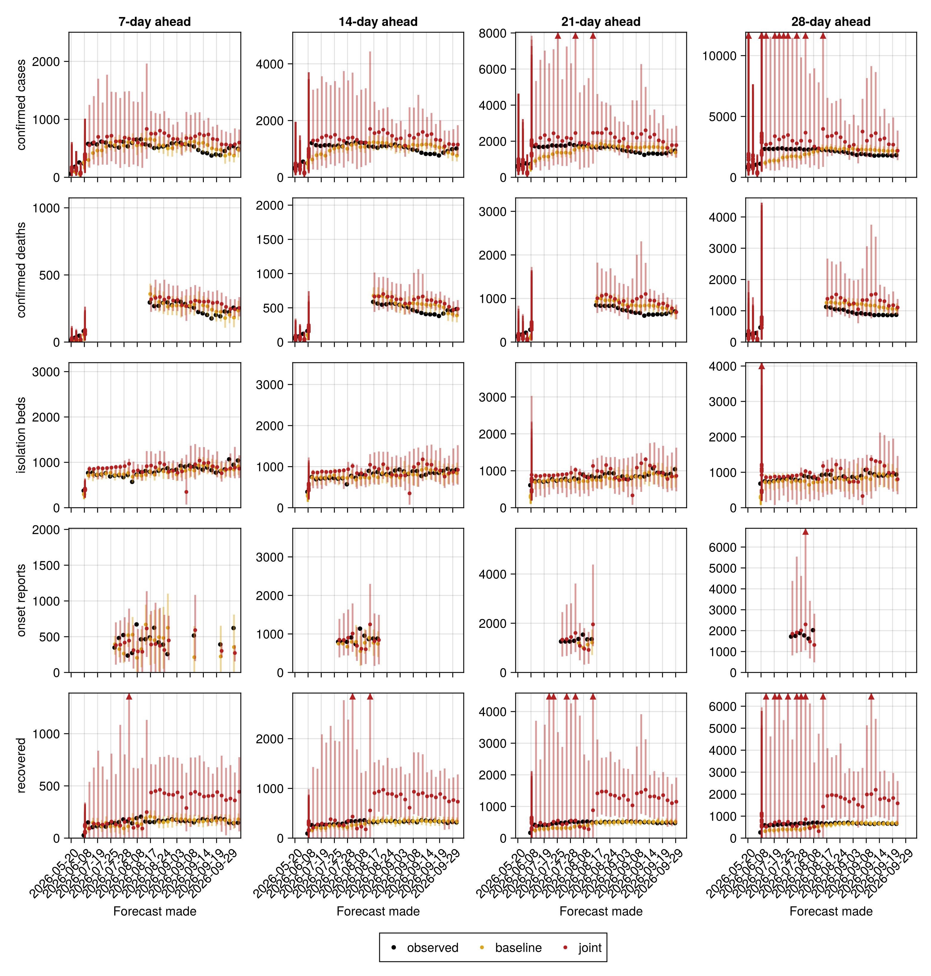
The frozen re-fits below freeze the renewal data to an earlier cut-off and re-fit, so that a change driven by newer data can be distinguished from one driven by a change of method. The one-week-back re-fit uses the headline sampler settings, and the re-fits at earlier cut-offs use the single-population frozen settings given in the methods.
Freeze the renewal data to a cut-off and re-fit
# Frozen re-fits and released_df are prepared in the setup block above.Individual fits against the baseline
This section scores each stream's own individual fit across releases, as forecast scoring across releases does the joint, against the same persistence baseline.
Individual-fit rows of the cross-release scores
# The relative skill against a stream's individual fit is only ever
# computed on the joint model's row, so on these rows it is missing by
# construction and the column is dropped rather than shown empty.
individual_score_overview_table = drop_individual_fit_columns(
    select_fit_role(forecast_score_overview_table, "individual")
)
individual_score_by_horizon_table = drop_individual_fit_columns(
    select_fit_role(forecast_score_by_horizon_table, "individual")
)
# See the comment above `joint_score_by_release_table`'s assignment for why
# this setup chunk's last statement needs a trailing `;`.
individual_score_by_release_table = drop_individual_fit_columns(
    select_fit_role(forecast_score_by_release_table, "individual")
);| stream | fit | n | crps | rel_to_baseline | log_crps | log_rel_to_baseline | dispersion | overprediction | underprediction | coverage_50 | coverage_90 | bias |
|---|---|---|---|---|---|---|---|---|---|---|---|---|
| confirmed cases | confirmed | 126 | 437.38 | 3.29 | 0.283 | 2.85 | 224.21 | 212.24 | 0.92 | 0.64 | 0.77 | 0.39 |
| confirmed deaths | confirmed_deaths | 126 | 204.32 | 2.34 | 0.366 | 2.97 | 152.44 | 18.1 | 33.78 | 0.73 | 1 | -0.12 |
| isolation beds | treatment | 126 | 112.3 | 1.95 | 0.156 | 2.17 | 101.16 | 0.56 | 10.57 | 0.98 | 1 | -0.14 |
| onset reports | onsets | 27 | 191.41 | 1.44 | 0.306 | 1.32 | 100 | 31.26 | 60.15 | 0.59 | 0.93 | -0.05 |
individual_relative_skill_fig = plot_forecast_relative_skill(
    individual_score_by_horizon_table;
    empty_message = "Empty: no release old enough for its targets to " *
        "have been observed carries an individual-stream " *
        "forecast. Not a missing forecast."
);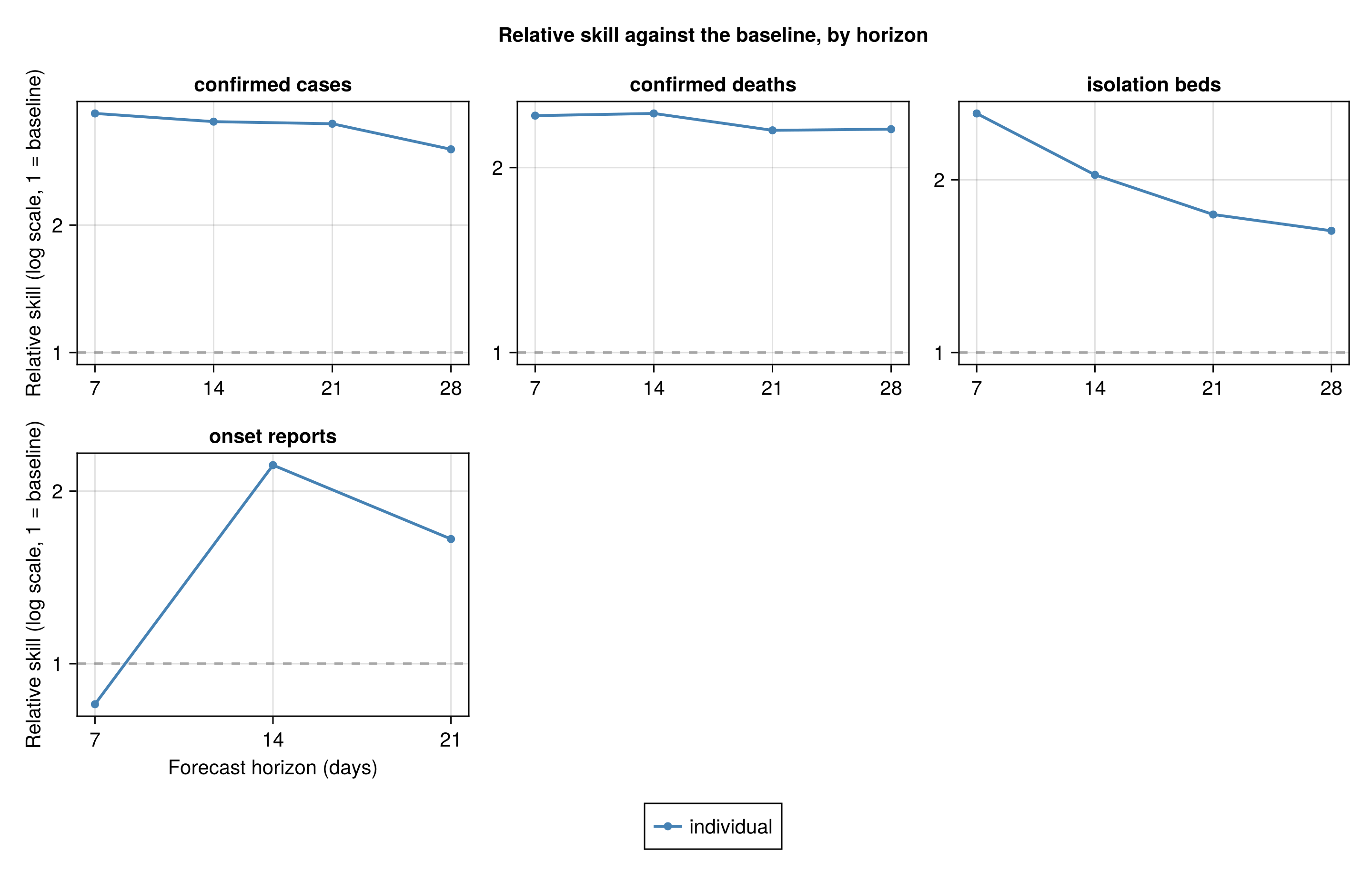
Scores by horizon
| stream | horizon | fit | n | crps | rel_to_baseline | log_crps | log_rel_to_baseline | dispersion | overprediction | underprediction | coverage_50 | coverage_90 | bias |
|---|---|---|---|---|---|---|---|---|---|---|---|---|---|
| confirmed cases | 7 | confirmed | 34 | 154.72 | 3.67 | 0.271 | 3.33 | 69.35 | 83.57 | 1.79 | 0.62 | 0.74 | 0.36 |
| confirmed cases | 14 | confirmed | 33 | 325.11 | 3.51 | 0.274 | 3.01 | 153.94 | 169.78 | 1.39 | 0.61 | 0.73 | 0.39 |
| confirmed cases | 21 | confirmed | 31 | 533.51 | 3.47 | 0.285 | 2.86 | 271.63 | 261.62 | 0.26 | 0.65 | 0.77 | 0.41 |
| confirmed cases | 28 | confirmed | 28 | 806.49 | 3.02 | 0.304 | 2.34 | 442.58 | 363.86 | 0.05 | 0.71 | 0.86 | 0.41 |
| confirmed deaths | 7 | confirmed_deaths | 34 | 60.25 | 2.43 | 0.327 | 3.46 | 39.84 | 2.61 | 17.8 | 0.65 | 1 | -0.17 |
| confirmed deaths | 14 | confirmed_deaths | 33 | 135.17 | 2.45 | 0.348 | 3.36 | 95.27 | 8.37 | 31.53 | 0.67 | 1 | -0.16 |
| confirmed deaths | 21 | confirmed_deaths | 31 | 241.97 | 2.3 | 0.378 | 2.89 | 180.35 | 19.09 | 42.52 | 0.74 | 1 | -0.12 |
| confirmed deaths | 28 | confirmed_deaths | 28 | 419.08 | 2.31 | 0.418 | 2.44 | 325.66 | 47.28 | 46.14 | 0.89 | 1 | -0.02 |
| isolation beds | 7 | treatment | 34 | 107.14 | 2.61 | 0.156 | 3.02 | 95.35 | 0.26 | 11.52 | 1 | 1 | -0.14 |
| isolation beds | 14 | treatment | 33 | 110.54 | 2.04 | 0.153 | 2.29 | 101.98 | 0.11 | 8.45 | 1 | 1 | -0.11 |
| isolation beds | 21 | treatment | 31 | 112.7 | 1.74 | 0.153 | 1.89 | 101.44 | 0.44 | 10.83 | 0.97 | 1 | -0.14 |
| isolation beds | 28 | treatment | 28 | 120.2 | 1.63 | 0.163 | 1.77 | 106.95 | 1.61 | 11.64 | 0.93 | 1 | -0.17 |
| onset reports | 7 | onsets | 13 | 100.92 | 0.85 | 0.35 | 1.06 | 63.66 | 14.44 | 22.83 | 0.77 | 0.85 | 0.08 |
| onset reports | 14 | onsets | 8 | 231.66 | 2.22 | 0.268 | 2.22 | 116.28 | 44.41 | 70.96 | 0.5 | 1 | -0.08 |
| onset reports | 21 | onsets | 6 | 333.79 | 1.65 | 0.26 | 1.61 | 157.03 | 50.16 | 126.59 | 0.33 | 1 | -0.28 |
Scores by release
| made_date | stream | fit | n | crps | rel_to_baseline | log_crps | log_rel_to_baseline | dispersion | overprediction | underprediction | coverage_50 | coverage_90 | bias |
|---|---|---|---|---|---|---|---|---|---|---|---|---|---|
| 2026-07-23 | confirmed cases | confirmed | 4 | 327.81 | 0.85 | 0.206 | 0.81 | 319.43 | 4.84 | 3.55 | 1 | 1 | -0.03 |
| 2026-07-25 | confirmed cases | confirmed | 4 | 346.24 | 1.49 | 0.213 | 1.51 | 343.88 | 2.3 | 0.06 | 1 | 1 | 0.02 |
| 2026-07-26 | confirmed cases | confirmed | 4 | 299.07 | 1.37 | 0.211 | 1.6 | 291.39 | 0.16 | 7.51 | 1 | 1 | -0.12 |
| 2026-07-27 | confirmed cases | confirmed | 4 | 267.62 | 1.31 | 0.171 | 1.25 | 262.03 | 5.38 | 0.21 | 1 | 1 | 0.04 |
| 2026-07-31 | confirmed cases | confirmed | 4 | 402.87 | 2.92 | 0.219 | 2.5 | 383.82 | 19.05 | 0 | 1 | 1 | 0.09 |
| 2026-08-01 | confirmed cases | confirmed | 4 | 336.31 | 2.83 | 0.209 | 2.92 | 322.98 | 13.33 | 0 | 1 | 1 | 0.08 |
| 2026-08-02 | confirmed cases | confirmed | 4 | 296.98 | 2.33 | 0.171 | 2.12 | 286.15 | 6.72 | 4.11 | 1 | 1 | -0.03 |
| 2026-08-03 | confirmed cases | confirmed | 4 | 291.8 | 1.53 | 0.175 | 1.23 | 281.42 | 10.08 | 0.3 | 1 | 1 | 0.05 |
| 2026-08-04 | confirmed cases | confirmed | 4 | 350.84 | 3.68 | 0.191 | 3.26 | 323.41 | 27.4 | 0.04 | 1 | 1 | 0.11 |
| 2026-08-07 | confirmed cases | confirmed | 4 | 308.4 | 3.6 | 0.192 | 2.79 | 294.77 | 9.51 | 4.12 | 1 | 1 | -0.01 |
| 2026-08-11 | confirmed cases | confirmed | 4 | 335.75 | 7.66 | 0.191 | 5.28 | 307.3 | 27.62 | 0.84 | 1 | 1 | 0.1 |
| 2026-08-15 | confirmed cases | confirmed | 4 | 312.22 | 5.3 | 0.211 | 4.19 | 308.06 | 1.82 | 2.34 | 1 | 1 | -0.03 |
| 2026-08-17 | confirmed cases | confirmed | 4 | 299.38 | 4.03 | 0.228 | 3.47 | 293.33 | 0 | 6.06 | 1 | 1 | -0.09 |
| 2026-08-22 | confirmed cases | confirmed | 4 | 335.33 | 4.91 | 0.206 | 4.06 | 293.02 | 42.31 | 0 | 1 | 1 | 0.15 |
| 2026-08-24 | confirmed cases | confirmed | 4 | 315.97 | 4.78 | 0.185 | 3.93 | 253.05 | 62.92 | 0 | 1 | 1 | 0.26 |
| 2026-08-25 | confirmed cases | confirmed | 4 | 302.15 | 4.47 | 0.184 | 3.98 | 236.93 | 65.23 | 0 | 1 | 1 | 0.27 |
| 2026-08-30 | confirmed cases | confirmed | 4 | 384.81 | 4.68 | 0.203 | 3.48 | 243.44 | 141.37 | 0 | 1 | 1 | 0.37 |
| 2026-08-31 | confirmed cases | confirmed | 4 | 298.73 | 3.12 | 0.177 | 2.81 | 219.12 | 79.61 | 0 | 1 | 1 | 0.26 |
| 2026-09-01 | confirmed cases | confirmed | 4 | 350.74 | 3.69 | 0.193 | 2.88 | 251.34 | 99.4 | 0 | 1 | 1 | 0.29 |
| 2026-09-06 | confirmed cases | confirmed | 4 | 352.02 | 2.8 | 0.215 | 2.76 | 256.32 | 95.71 | 0 | 1 | 1 | 0.33 |
| 2026-09-10 | confirmed cases | confirmed | 4 | 448.08 | 2.46 | 0.264 | 2.02 | 245.86 | 202.22 | 0 | 0.25 | 1 | 0.48 |
| 2026-09-12 | confirmed cases | confirmed | 4 | 1307.03 | 5.17 | 0.747 | 3.77 | 117.75 | 1189.28 | 0 | 0 | 0 | 1 |
| 2026-09-13 | confirmed cases | confirmed | 4 | 1202.65 | 5.78 | 0.694 | 4.27 | 121.72 | 1080.92 | 0 | 0 | 0 | 1 |
| 2026-09-15 | confirmed cases | confirmed | 4 | 1039.06 | 4.56 | 0.657 | 3.31 | 126.86 | 912.21 | 0 | 0 | 0 | 1 |
| 2026-09-16 | confirmed cases | confirmed | 4 | 948 | 4.45 | 0.617 | 3.4 | 127.78 | 820.22 | 0 | 0 | 0 | 1 |
| 2026-09-19 | confirmed cases | confirmed | 4 | 650.67 | 3.35 | 0.482 | 2.92 | 126.04 | 524.63 | 0 | 0 | 0.25 | 0.95 |
| 2026-09-21 | confirmed cases | confirmed | 4 | 480.05 | 4.97 | 0.366 | 4.83 | 100.45 | 379.61 | 0 | 0 | 0.25 | 0.94 |
| 2026-09-22 | confirmed cases | confirmed | 4 | 356.78 | 4.66 | 0.287 | 4.97 | 112.6 | 244.18 | 0 | 0 | 0.5 | 0.9 |
| 2026-09-25 | confirmed cases | confirmed | 3 | 308.38 | 6.72 | 0.279 | 4.25 | 74.77 | 233.6 | 0 | 0 | 0.33 | 0.91 |
| 2026-09-26 | confirmed cases | confirmed | 3 | 380.88 | 10.33 | 0.378 | 8.27 | 67.39 | 313.49 | 0 | 0 | 0 | 0.96 |
| 2026-09-27 | confirmed cases | confirmed | 3 | 212.42 | 4.13 | 0.19 | 2.44 | 72.52 | 139.9 | 0 | 0 | 1 | 0.81 |
| 2026-10-02 | confirmed cases | confirmed | 2 | 123.67 | 2.15 | 0.155 | 2.03 | 42.61 | 81.06 | 0 | 0 | 1 | 0.82 |
| 2026-10-06 | confirmed cases | confirmed | 2 | 135.84 | 4.19 | 0.162 | 3.7 | 45.71 | 90.13 | 0 | 0 | 1 | 0.77 |
| 2026-10-10 | confirmed cases | confirmed | 1 | 96.01 | 2.46 | 0.173 | 2.29 | 29.23 | 66.78 | 0 | 0 | 1 | 0.79 |
| 2026-07-23 | confirmed deaths | confirmed_deaths | 4 | 701.54 | 4.32 | 0.448 | 2.27 | 383.29 | 318.25 | 0 | 0.25 | 1 | 0.56 |
| 2026-07-25 | confirmed deaths | confirmed_deaths | 4 | 237.78 | 1.79 | 0.234 | 1.44 | 214.28 | 23.5 | 0 | 1 | 1 | 0.18 |
| 2026-07-26 | confirmed deaths | confirmed_deaths | 4 | 256.46 | 2.27 | 0.255 | 1.99 | 231.65 | 24.81 | 0 | 1 | 1 | 0.13 |
| 2026-07-27 | confirmed deaths | confirmed_deaths | 4 | 310.27 | 2.77 | 0.252 | 1.82 | 280.84 | 29.43 | 0 | 1 | 1 | 0.21 |
| 2026-07-31 | confirmed deaths | confirmed_deaths | 4 | 312.36 | 2.62 | 0.289 | 2.04 | 292.21 | 20.08 | 0.07 | 1 | 1 | 0.08 |
| 2026-08-01 | confirmed deaths | confirmed_deaths | 4 | 280.92 | 2.38 | 0.253 | 1.67 | 261.46 | 19.46 | 0 | 1 | 1 | 0.1 |
| 2026-08-02 | confirmed deaths | confirmed_deaths | 4 | 256.05 | 2.85 | 0.276 | 2.47 | 238.23 | 16.88 | 0.94 | 1 | 1 | 0.03 |
| 2026-08-03 | confirmed deaths | confirmed_deaths | 4 | 224.5 | 1.72 | 0.245 | 1.29 | 212.2 | 10.83 | 1.46 | 1 | 1 | 0.02 |
| 2026-08-04 | confirmed deaths | confirmed_deaths | 4 | 248.77 | 3.56 | 0.283 | 3.43 | 242.12 | 4.29 | 2.35 | 1 | 1 | -0.02 |
| 2026-08-07 | confirmed deaths | confirmed_deaths | 4 | 231.5 | 3.3 | 0.325 | 3.17 | 223.68 | 1.02 | 6.79 | 1 | 1 | -0.11 |
| 2026-08-11 | confirmed deaths | confirmed_deaths | 4 | 244.6 | 12.23 | 0.337 | 11.68 | 233.59 | 1.95 | 9.06 | 1 | 1 | -0.13 |
| 2026-08-15 | confirmed deaths | confirmed_deaths | 4 | 244.83 | 5.94 | 0.34 | 5.47 | 239.91 | 0.04 | 4.89 | 1 | 1 | -0.1 |
| 2026-08-17 | confirmed deaths | confirmed_deaths | 4 | 251.32 | 4.34 | 0.297 | 3.49 | 246.09 | 3.93 | 1.3 | 1 | 1 | -0.02 |
| 2026-08-22 | confirmed deaths | confirmed_deaths | 4 | 242 | 2.54 | 0.482 | 3.76 | 219.73 | 0 | 22.27 | 1 | 1 | -0.18 |
| 2026-08-24 | confirmed deaths | confirmed_deaths | 4 | 220.02 | 2.99 | 0.543 | 6.03 | 144.48 | 0 | 75.54 | 1 | 1 | -0.4 |
| 2026-08-25 | confirmed deaths | confirmed_deaths | 4 | 247.19 | 3.4 | 0.796 | 9.42 | 151.31 | 0 | 95.88 | 0.75 | 1 | -0.45 |
| 2026-08-30 | confirmed deaths | confirmed_deaths | 4 | 260.37 | 3.17 | 0.907 | 9.9 | 129.82 | 0 | 130.55 | 0.5 | 1 | -0.51 |
| 2026-08-31 | confirmed deaths | confirmed_deaths | 4 | 247.04 | 2.18 | 0.782 | 5.82 | 144.82 | 0 | 102.22 | 1 | 1 | -0.4 |
| 2026-09-01 | confirmed deaths | confirmed_deaths | 4 | 246.66 | 2.55 | 0.927 | 8.12 | 116.86 | 0 | 129.8 | 0.5 | 1 | -0.48 |
| 2026-09-06 | confirmed deaths | confirmed_deaths | 4 | 281.88 | 3.01 | 1.171 | 10.51 | 79.51 | 0 | 202.37 | 0 | 1 | -0.64 |
| 2026-09-10 | confirmed deaths | confirmed_deaths | 4 | 207.51 | 1.57 | 0.746 | 3.78 | 124.24 | 0 | 83.27 | 0.75 | 1 | -0.45 |
| 2026-09-12 | confirmed deaths | confirmed_deaths | 4 | 100.94 | 0.72 | 0.15 | 0.66 | 60.06 | 40.87 | 0 | 0.25 | 1 | 0.54 |
| 2026-09-13 | confirmed deaths | confirmed_deaths | 4 | 94.04 | 0.78 | 0.145 | 0.76 | 55.49 | 38.55 | 0 | 0.25 | 1 | 0.57 |
| 2026-09-15 | confirmed deaths | confirmed_deaths | 4 | 62.49 | 0.52 | 0.108 | 0.53 | 52.89 | 9.6 | 0 | 1 | 1 | 0.31 |
| 2026-09-16 | confirmed deaths | confirmed_deaths | 4 | 57.36 | 0.56 | 0.102 | 0.58 | 52.38 | 4.98 | 0 | 0.75 | 1 | 0.26 |
| 2026-09-19 | confirmed deaths | confirmed_deaths | 4 | 54.29 | 0.61 | 0.095 | 0.65 | 48.66 | 1.3 | 4.32 | 1 | 1 | 0.01 |
| 2026-09-21 | confirmed deaths | confirmed_deaths | 4 | 44.17 | 0.77 | 0.08 | 0.88 | 31.16 | 0.2 | 12.8 | 1 | 1 | -0.2 |
| 2026-09-22 | confirmed deaths | confirmed_deaths | 4 | 68.07 | 1.6 | 0.121 | 1.82 | 27.69 | 0 | 40.38 | 0.5 | 1 | -0.51 |
| 2026-09-25 | confirmed deaths | confirmed_deaths | 3 | 91.91 | 3 | 0.228 | 2.47 | 20.35 | 0 | 71.56 | 0 | 1 | -0.82 |
| 2026-09-26 | confirmed deaths | confirmed_deaths | 3 | 48.01 | 2 | 0.109 | 1.88 | 20.64 | 0.23 | 27.14 | 0.33 | 1 | -0.39 |
| 2026-09-27 | confirmed deaths | confirmed_deaths | 3 | 62.67 | 2.86 | 0.149 | 2.47 | 20.1 | 0 | 42.57 | 0 | 1 | -0.65 |
| 2026-10-02 | confirmed deaths | confirmed_deaths | 2 | 43.18 | 2.14 | 0.142 | 2.43 | 14.79 | 0 | 28.39 | 0 | 1 | -0.72 |
| 2026-10-06 | confirmed deaths | confirmed_deaths | 2 | 47.97 | 2.17 | 0.148 | 2.37 | 14.74 | 0 | 33.23 | 0 | 1 | -0.79 |
| 2026-10-10 | confirmed deaths | confirmed_deaths | 1 | 14.38 | 0.71 | 0.069 | 0.84 | 10.79 | 0 | 3.59 | 1 | 1 | -0.32 |
| 2026-07-23 | isolation beds | treatment | 4 | 55.73 | 1.89 | 0.089 | 2.3 | 47.79 | 0 | 7.94 | 1 | 1 | -0.21 |
| 2026-07-25 | isolation beds | treatment | 4 | 51.68 | 1.32 | 0.082 | 1.58 | 47.14 | 0.01 | 4.52 | 1 | 1 | -0.14 |
| 2026-07-26 | isolation beds | treatment | 4 | 61.67 | 1.55 | 0.1 | 1.86 | 54.82 | 0.23 | 6.63 | 1 | 1 | -0.12 |
| 2026-07-27 | isolation beds | treatment | 4 | 59.47 | 2.18 | 0.098 | 2.66 | 54.67 | 0 | 4.8 | 1 | 1 | -0.18 |
| 2026-07-31 | isolation beds | treatment | 4 | 82.76 | 2.01 | 0.132 | 2.5 | 68.17 | 0 | 14.6 | 0.75 | 1 | -0.28 |
| 2026-08-01 | isolation beds | treatment | 4 | 88.62 | 1.38 | 0.153 | 1.78 | 73.94 | 0 | 14.67 | 0.75 | 1 | -0.25 |
| 2026-08-02 | isolation beds | treatment | 4 | 84.37 | 1.59 | 0.141 | 1.96 | 69.7 | 0 | 14.67 | 0.75 | 1 | -0.28 |
| 2026-08-03 | isolation beds | treatment | 4 | 79.93 | 1.96 | 0.134 | 2.42 | 71.91 | 0 | 8.01 | 1 | 1 | -0.21 |
| 2026-08-04 | isolation beds | treatment | 4 | 87.06 | 1.35 | 0.141 | 1.53 | 82.73 | 1.22 | 3.11 | 1 | 1 | -0.03 |
| 2026-08-07 | isolation beds | treatment | 4 | 104.98 | 1.56 | 0.171 | 1.94 | 85.76 | 0 | 19.21 | 1 | 1 | -0.29 |
| 2026-08-11 | isolation beds | treatment | 4 | 102.61 | 0.59 | 0.171 | 0.68 | 90.93 | 0 | 11.68 | 1 | 1 | -0.21 |
| 2026-08-15 | isolation beds | treatment | 4 | 127.51 | 1.46 | 0.204 | 1.85 | 98.57 | 0 | 28.94 | 1 | 1 | -0.33 |
| 2026-08-17 | isolation beds | treatment | 4 | 103.76 | 1.39 | 0.161 | 1.67 | 93.32 | 0 | 10.44 | 1 | 1 | -0.19 |
| 2026-08-22 | isolation beds | treatment | 4 | 144.98 | 2.73 | 0.218 | 3.39 | 120.25 | 0 | 24.73 | 1 | 1 | -0.22 |
| 2026-08-24 | isolation beds | treatment | 4 | 127.24 | 2.62 | 0.181 | 3.01 | 115.13 | 1.05 | 11.06 | 1 | 1 | -0.11 |
| 2026-08-25 | isolation beds | treatment | 4 | 131.92 | 1.82 | 0.191 | 2.11 | 111.86 | 0 | 20.06 | 1 | 1 | -0.2 |
| 2026-08-30 | isolation beds | treatment | 4 | 128.62 | 2.92 | 0.171 | 3.13 | 117.42 | 5.73 | 5.47 | 1 | 1 | -0.02 |
| 2026-08-31 | isolation beds | treatment | 4 | 120.61 | 2.82 | 0.16 | 3.12 | 111.75 | 1.79 | 7.07 | 1 | 1 | -0.07 |
| 2026-09-01 | isolation beds | treatment | 4 | 120.7 | 2.93 | 0.154 | 3.24 | 116.43 | 0.68 | 3.6 | 1 | 1 | -0.05 |
| 2026-09-06 | isolation beds | treatment | 4 | 124.13 | 2.49 | 0.156 | 2.58 | 120.73 | 1.81 | 1.58 | 1 | 1 | -0.01 |
| 2026-09-10 | isolation beds | treatment | 4 | 129.27 | 2.55 | 0.158 | 2.64 | 119.72 | 0.24 | 9.31 | 1 | 1 | -0.06 |
| 2026-09-12 | isolation beds | treatment | 4 | 134.16 | 2.24 | 0.181 | 2.69 | 121.99 | 0 | 12.16 | 1 | 1 | -0.13 |
| 2026-09-13 | isolation beds | treatment | 4 | 121.64 | 2.21 | 0.157 | 2.53 | 120.42 | 0.02 | 1.2 | 1 | 1 | -0.04 |
| 2026-09-15 | isolation beds | treatment | 4 | 132.57 | 2.43 | 0.16 | 2.74 | 125.5 | 0.31 | 6.75 | 1 | 1 | -0.06 |
| 2026-09-16 | isolation beds | treatment | 4 | 130.44 | 3.26 | 0.16 | 3.62 | 123.53 | 0.2 | 6.7 | 1 | 1 | -0.1 |
| 2026-09-19 | isolation beds | treatment | 4 | 126.15 | 2.41 | 0.149 | 2.48 | 124.25 | 1.85 | 0.05 | 1 | 1 | 0.03 |
| 2026-09-21 | isolation beds | treatment | 4 | 136.46 | 2.39 | 0.155 | 2.35 | 134.53 | 1.03 | 0.91 | 1 | 1 | 0.01 |
| 2026-09-22 | isolation beds | treatment | 4 | 182.97 | 2.62 | 0.243 | 3.22 | 143.66 | 0 | 39.32 | 1 | 1 | -0.26 |
| 2026-09-25 | isolation beds | treatment | 3 | 131.32 | 2.61 | 0.151 | 2.52 | 127.47 | 2.09 | 1.76 | 1 | 1 | -0.01 |
| 2026-09-26 | isolation beds | treatment | 3 | 118.86 | 1.51 | 0.142 | 1.49 | 112.75 | 0.05 | 6.06 | 1 | 1 | -0.09 |
| 2026-09-27 | isolation beds | treatment | 3 | 139.64 | 2 | 0.179 | 2.13 | 126.23 | 0 | 13.4 | 1 | 1 | -0.17 |
| 2026-10-02 | isolation beds | treatment | 2 | 125.25 | 2.27 | 0.15 | 2.37 | 120.52 | 0 | 4.73 | 1 | 1 | -0.12 |
| 2026-10-06 | isolation beds | treatment | 2 | 139.19 | 1.93 | 0.166 | 2.31 | 110.52 | 0 | 28.67 | 1 | 1 | -0.29 |
| 2026-10-10 | isolation beds | treatment | 1 | 123.47 | 4.6 | 0.146 | 5.14 | 118.47 | 0 | 5 | 1 | 1 | -0.12 |
| 2026-08-02 | onset reports | onsets | 3 | 122.9 | 0.9 | 0.188 | 1.13 | 96.84 | 0 | 26.06 | 1 | 1 | -0.28 |
| 2026-08-03 | onset reports | onsets | 3 | 105.39 | 1.59 | 0.166 | 1.28 | 100.32 | 1.15 | 3.92 | 1 | 1 | -0.02 |
| 2026-08-04 | onset reports | onsets | 3 | 141.84 | 1.11 | 0.266 | 1.22 | 88.34 | 0.04 | 53.46 | 0.67 | 1 | -0.26 |
| 2026-08-07 | onset reports | onsets | 3 | 378.48 | 1.14 | 0.633 | 1.39 | 82.32 | 0 | 296.16 | 0 | 1 | -0.8 |
| 2026-08-11 | onset reports | onsets | 3 | 243.78 | 1.42 | 0.429 | 1.69 | 85.91 | 0 | 157.87 | 0.33 | 1 | -0.64 |
| 2026-08-15 | onset reports | onsets | 3 | 369.23 | 4.41 | 0.277 | 2.54 | 205.04 | 164.18 | 0 | 0.33 | 1 | 0.57 |
| 2026-08-17 | onset reports | onsets | 2 | 246.49 | 4 | 0.255 | 2.25 | 153.61 | 92.88 | 0 | 0.5 | 1 | 0.47 |
| 2026-08-22 | onset reports | onsets | 2 | 120.98 | 1.15 | 0.21 | 1.39 | 104.12 | 16.87 | 0 | 1 | 1 | 0.22 |
| 2026-08-24 | onset reports | onsets | 1 | 85.16 | 1.24 | 0.392 | 2.5 | 82.09 | 0 | 3.07 | 1 | 1 | -0.12 |
| 2026-08-25 | onset reports | onsets | 1 | 95.66 | 0.4 | 0.511 | 0.86 | 88.57 | 7.09 | 0 | 1 | 1 | 0.18 |
| 2026-09-21 | onset reports | onsets | 1 | 72.06 | 1.12 | 0.236 | 0.76 | 10.97 | 61.09 | 0 | 0 | 0 | 0.98 |
| 2026-09-22 | onset reports | onsets | 1 | 72.99 | 1.24 | 0.237 | 0.56 | 12.83 | 60.16 | 0 | 0 | 0 | 0.98 |
| 2026-10-02 | onset reports | onsets | 1 | 22.28 | 0.34 | 0.077 | 0.34 | 13.71 | 0 | 8.57 | 1 | 1 | -0.43 |
Saving forecast outputs
The one-week-back validation forecast is written in the release forecast's archive format, so it is recorded as a release asset alongside the forecast it is scored against.
Write forecast outputs
output_dir = get(
    ENV, "BVD_OUTPUT_DIR",
    joinpath(pkgdir(BVDOutbreakSize), "output")
)
mkpath(output_dir)
CSV.write(
    joinpath(output_dir, "forecast_validation.csv"),
    forecast_archive(
        [(7, validation_forecast)];
        made_date = frozen_lastweek.o.cutoff, thin = 5
    )
)"/home/runner/work/BVDOutbreakSize/BVDOutbreakSize/output/forecast_validation.csv"Write the summary bullets
# The bullets under the summary heading at the top of the page. They read
# tables built further down, so they are written here and read back when
# the site is assembled.
evaluation_forecast_national_summary = let
    fmt(x) = ismissing(x) || !isfinite(x) ? "n/a" :
        string(round(x; digits = 2))
    scored(tbl) = filter(r -> !ismissing(r.rel_to_baseline), tbl)
    function beat(label, tbl)
        rows = scored(tbl)
        size(rows, 1) == 0 &&
            return string("- **", label, ":** no scored forecasts yet.")
        return string(
            "- **", label, ":** beat the baseline on ",
            count(<(1), rows.rel_to_baseline), " of ", size(rows, 1),
            " streams."
        )
    end
    function block(lead, tbl)
        rows = scored(tbl)
        size(rows, 1) == 0 && return nothing
        return join(
            vcat(
                [string("**", lead, "**"), ""],
                [
                    string(
                        "- ", r.stream, ": relative skill ",
                        fmt(r.rel_to_baseline), ", 90% coverage ",
                        fmt(r.coverage_90), ", bias ", fmt(r.bias), " over ",
                        r.n, " forecasts."
                    )
                        for r in eachrow(rows)
                ]
            ), "\n"
        )
    end
    frozen_joint = select_fit_role(frozen_score_overview_table, "joint")
    overall = [
        beat("Joint model across releases", joint_score_overview_table),
        beat("Frozen joint model", frozen_joint),
    ]
    blocks = filter(
        !isnothing,
        [
            block("Across releases", joint_score_overview_table),
            block("Frozen fits", frozen_joint),
        ]
    )
    join(vcat([join(overall, "\n")], blocks), "\n\n")
end
dashboard_dir = joinpath(
    pkgdir(BVDOutbreakSize), "docs", "src", "summary_assets"
)
mkpath(dashboard_dir)
write(
    joinpath(dashboard_dir, "evaluation_forecast_national.md"),
    evaluation_forecast_national_summary
);