In-sample checks
This page checks whether the joint model reproduces the national data it was fitted to. It also compares the single-stream fits with the joint, breaks the sampler diagnostics down by parameter, refits the joint under alternative assumptions and sets the current estimates against past releases. The same checks by province are on the province in-sample checks page and by health zone on the health-zone in-sample checks page. How the model predicts data it has not seen is on the forecast evaluation page.
Load packages, data and fitted chains
# Shared setup: packages, observations and the fit registry. See
# `docs/pages/_setup.jl`.
using BVDOutbreakSize
include(joinpath(pkgdir(BVDOutbreakSize), "docs", "pages", "_setup.jl"))
validation_forecast_from (generic function with 1 method)# The fits and prior draws this page reads, loaded from the cache here.
chn_joint = load_fit("joint")
prior_chn = joint_prior_draws()
# `sens_no_patches` is the headline with `n_patches = 1`, the check on the
# spatial structure.
chn_no_patches = load_fit("sens_no_patches")
chn_exports = load_fit("exports")
chn_deaths = load_fit("deaths")
chn_cases = load_fit("cases")
chn_confirmed = load_fit("confirmed")
chn_confirmed_deaths = load_fit("confirmed_deaths")
chn_treatment = load_fit("treatment")
chn_onsets = load_fit("onsets")
frozen_lastweek = load_fit("frozen_validation")
# The frozen joint fits at earlier cut-offs, for the estimates across
# releases.
frozen_by_cutoff = frozen_fits_by_cutoff()
frozen_C(c) = vec(Array(frozen_by_cutoff[c].chn[:C_T]))
# Every frozen fit is a full joint fit, so it carries the same walk base
# chn_joint does.
frozen_R0(c) = r0_walk_draws(frozen_by_cutoff[c].chn)
if RUN_SENSITIVITY
chn_joint_community_delay = load_fit("sens_community_delay")
chn_joint_exp_growth_clock = load_fit("sens_exp_growth_clock")
end
posterior_C_joint = vec(Array(chn_joint[:C_T]))
posterior_C_exports = vec(Array(chn_exports[:C_T]))
posterior_C_deaths = vec(Array(chn_deaths[:C_T]))
posterior_C_cases = vec(Array(chn_cases[:C_T]))
posterior_C_confirmed = vec(Array(chn_confirmed[:C_T]))
posterior_C_treatment = vec(Array(chn_treatment[:C_T]))
posterior_C_onsets = vec(Array(chn_onsets[:C_T]));Summary
Whether each stream is reproduced, from the checks below. Bias runs from −1 to 1 and is negative when the model under-predicts, and coverage is the fraction of vintages inside the predictive interval.
Streams: 11 of 17 fitted streams have 90% coverage of at least 0.8.
Least well reproduced: Specimens analysed (cumulative) (bias -0.16, 90% coverage 0.5); In-care deaths/day (bias 0.14, 90% coverage 0.81); New suspected deaths/day (bias -0.11, 90% coverage 0.94).
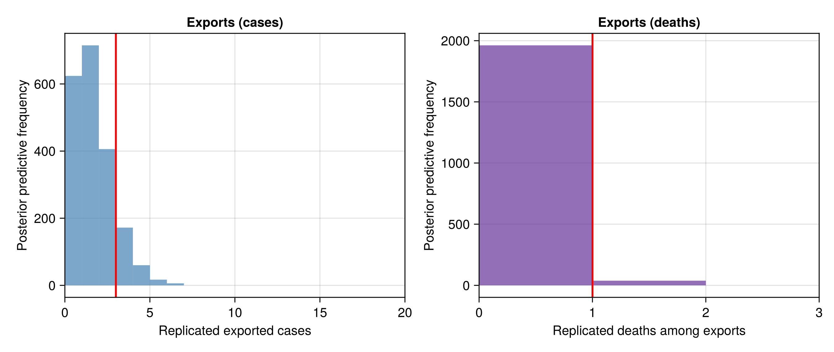
Exports: Uganda exports observed 3 against a predictive median of 1 (90% interval 0–3), and export deaths observed 1 against a predictive median of 0 (90% interval 0–0).
Streams still reporting
New suspects/day: bias 0.02, 90% coverage 0.94 over 129 vintages.
Patients in isolation: bias 0.01, 90% coverage 0.94 over 90 vintages.
Confirmed cases: bias 0.07, 90% coverage 0.92 over 149 vintages.
Confirmed deaths: bias 0.03, 90% coverage 0.89 over 151 vintages.
Recovered (confirmed): bias 0.02, 90% coverage 0.92 over 130 vintages.
Specimens analysed (24h): bias -0.04, 90% coverage 0.98 over 132 vintages.
Streams no longer reporting
Suspected cases: bias -0.01, 90% coverage 0.67 over 9 vintages.
Suspected deaths: bias -0.04, 90% coverage 0.78 over 9 vintages.
New suspected deaths/day: bias -0.11, 90% coverage 0.94 over 32 vintages.
Specimens analysed (cumulative): bias -0.16, 90% coverage 0.5 over 6 vintages.
Admissions/day: bias 0.08, 90% coverage 0.74 over 42 vintages.
In-care deaths/day: bias 0.14, 90% coverage 0.81 over 42 vintages.
Rule-outs/day: bias -0.02, 90% coverage 0.56 over 41 vintages.
Absconded/day: bias 0.09, 90% coverage 0.83 over 42 vintages.
Confirmed in care: bias -0.04, 90% coverage 1.0 over 38 vintages.
Suspects in care: bias -0.06, 90% coverage 0.92 over 38 vintages.
Onset reports (net correction/snapshot): bias -0.11, 90% coverage 0.68 over 59 vintages.
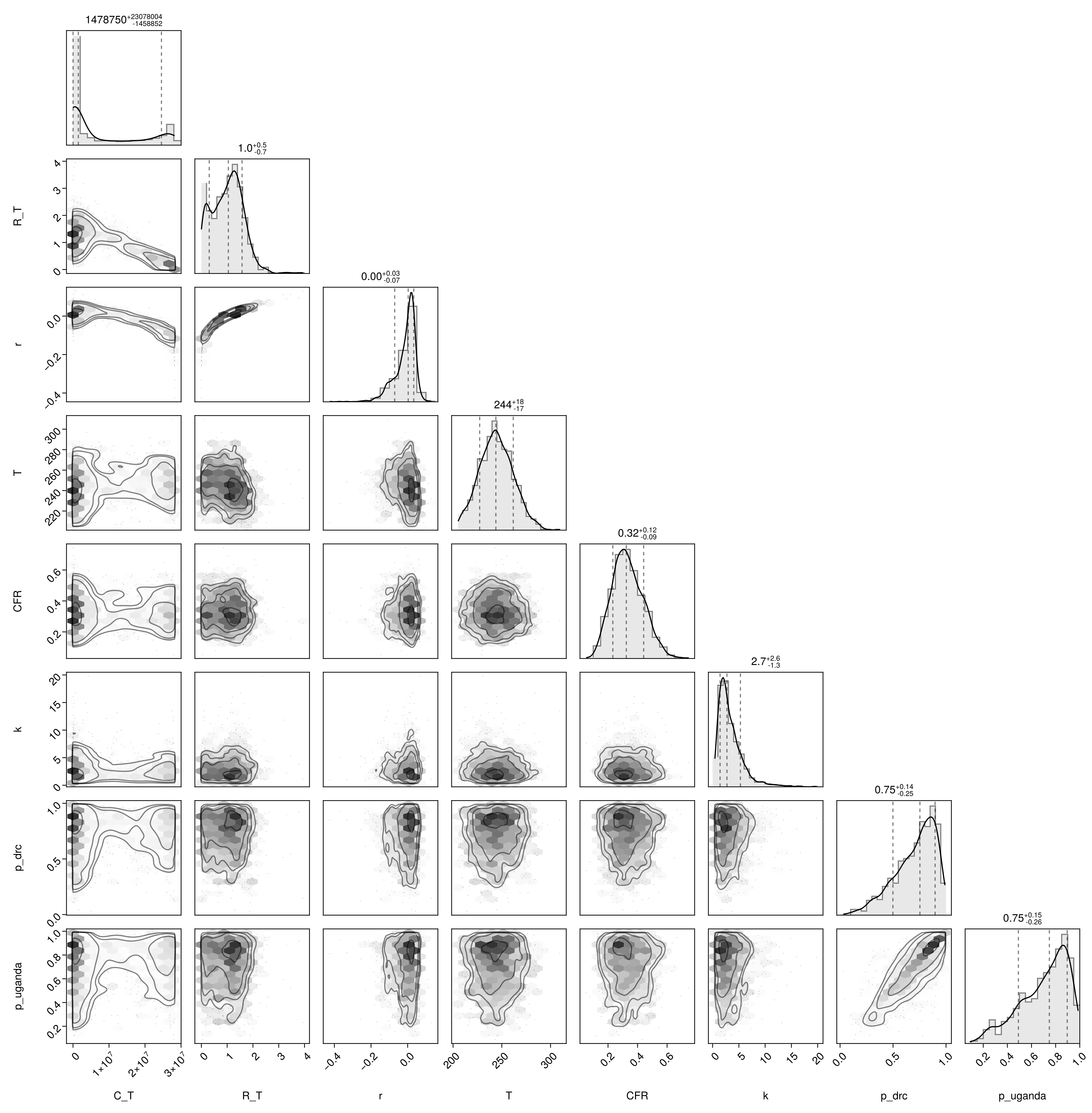
Prior predictive check
Whether the prior, before any data are fitted, brackets the observed counts.
Summarise the joint prior
prior_C_table = summary_table(prior_chn, [:C_T]; digits = 0);Show prior summary table
| Row | Quantity | Lower 90% | Lower 60% | Lower 30% | Upper 30% | Upper 60% | Upper 90% |
|---|---|---|---|---|---|---|---|
| String | Float64 | Float64 | Float64 | Float64 | Float64 | Float64 | |
| 1 | C_T | 2949.0 | 29583.0 | 204588.0 | 8.78809e6 | 2.2505e7 | 2.75879e7 |
Prior pair plot
prior_pair_fig = plot_pair(
    prior_chn,
    [
        :C_T, :R_T, :r, :T, :CFR, :k,
        :p_drc, :p_uganda,
    ]
);
Posterior predictive checks
Whether data replicated from the fitted model reproduce each observed stream.
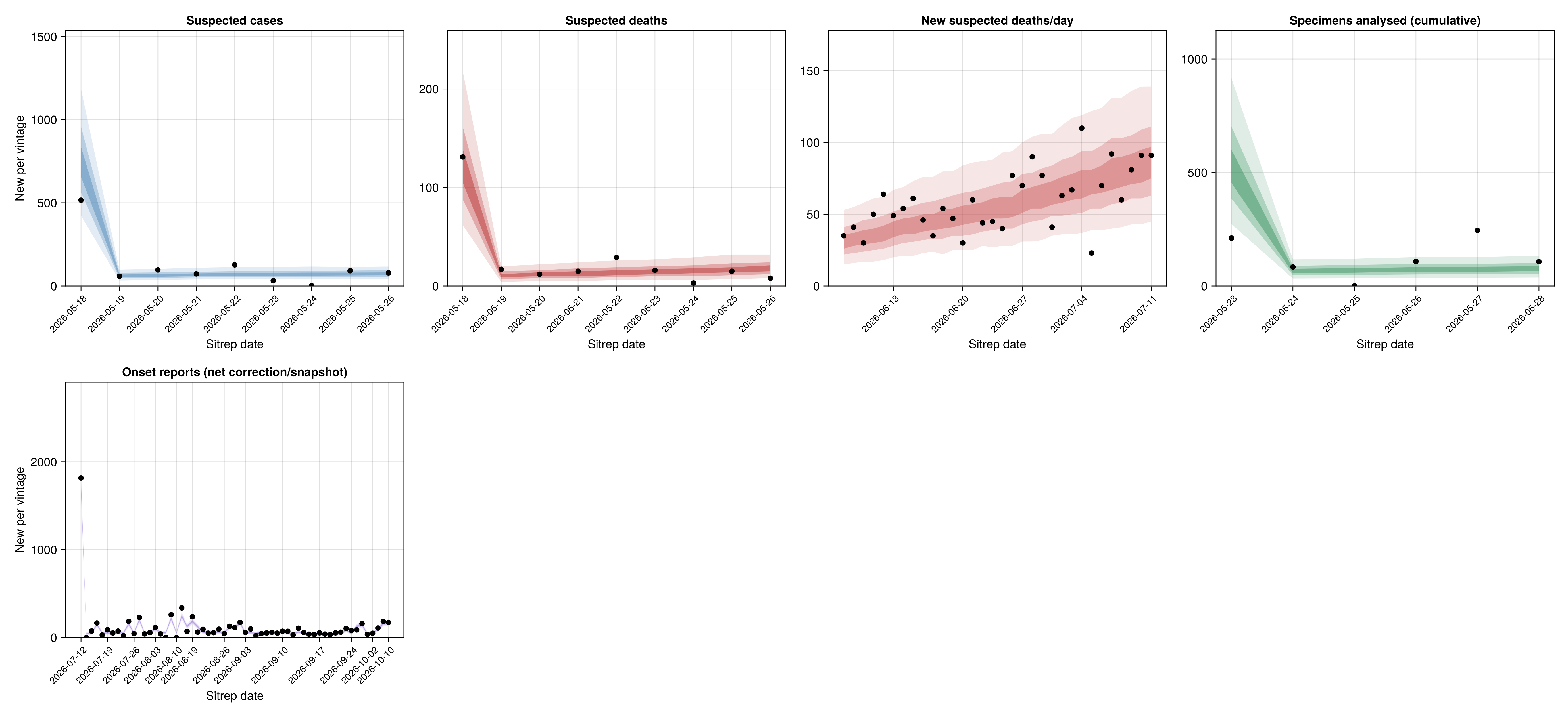
Streams still reporting
Whether the streams reported within a week of the cut-off are reproduced.
Cumulative
Whether the replicated running totals, or daily counts for a daily stream, track the observed ones.
Joint posterior predictive plot
# The joint posterior predictive, shared with the province page (see
# `joint_posterior_predictive` in `docs/pages/_setup.jl`).
pp_joint = joint_posterior_predictive();

# `predict` stores each stream's per-vintage increments as one
# vector-valued variable (`<stream>_increments.increments`); the slice is
# an iter×chain matrix of per-draw increment vectors, exactly the
# `replicates` shape `plot_vintage_conditional_ppc` grounds on each
# vintage's observed previous cumulative for the one-step-ahead
# predictive. Look it up by its VarName with FlexiChains' `Prefixed`, which
# matches a (submodel-prefixed) key by its varname tail: `Prefixed(@varname(
# reported_increments.increments))` finds `cases_state.reported_increments.
# increments` without hard-coding the `cases_state.` prefix, and matches by
# the varname tail rather than a loose substring, so it cannot be fooled by a
# scalar `expected_*_T` deterministic. `FlexiChains` is a package
# dependency (imported, not exported), so it is reached through the package
# namespace.
const _Prefixed = BVDOutbreakSize.FlexiChains.Prefixed;
_vintage_replicates(pp, vn) = collect(pp[_Prefixed(vn)]);

# Grid day-index → INSP situation-report date label.
_vintage_dates(days) = string.(obs.seeding .+ Day.(days .- 1));

reported_panel = (;
    id = :suspected_cases,
    title = "Suspected cases",
    dates = _vintage_dates(obs.reported_history.days),
    replicates = _vintage_replicates(
        pp_joint, @varname(reported_increments.increments)
    ),
    observed = obs.reported_history.counts, colour = :steelblue,
);
# Daily new-suspect inflow: a per-day count (not cumulative), so the panel
# is drawn with `cumulative = false` — each replicate is its own daily
# count against the observed daily count rather than a running total. Its
# days pick up where the cumulative suspected panel freezes.
suspected_daily_panel = (;
    id = :suspected_daily,
    title = "New suspects/day",
    dates = _vintage_dates(obs.suspected_daily_history.days),
    replicates = _vintage_replicates(
        pp_joint, @varname(suspected_daily.increments)
    ),
    observed = obs.suspected_daily_history.counts,
    colour = :slateblue, cumulative = false,
);
# Isolation/treatment-bed occupancy: a census stock, so the panel is drawn
# with `cumulative = false` — each replicate is the modelled bed count on a
# report day against the observed "Patients en isolement" count. It is a
# level, not a count of new events, so it carries its own `ylabel` rather
# than the "Daily count" and "New per vintage" defaults, which would read as
# an accumulating total on a series that rises through the outbreak. The count
# is the suspect inflow carried through a length-of-stay survival, so its
# level and lag reflect the admission proportion and the stays. The censored-
# occupancy likelihood stores its per-day predictive draws under the submodel
# `obs` variable (not `increments`), so the replicates are read from that key.
# The treatment model scores the total occupancy only on the days without a
# published confirmed/suspect split (a per-day total-or-split switch): on the
# split days the two sub-stock census panels carry the fit instead, so the
# `isolation.obs` predictive holds only the non-split days. Drop the split
# days from the panel's dates and observed counts to match that length.
_iso_split_days = Set(Int.(obs.treatment_confirmed_incare_history.days))
_iso_keep = [!(Int(d) in _iso_split_days) for d in obs.isolation_history.days]
isolation_panel = (;
    id = :isolation_beds,
    title = "Patients in isolation",
    dates = _vintage_dates(obs.isolation_history.days[_iso_keep]),
    replicates = _vintage_replicates(
        pp_joint, @varname(isolation.obs)
    ),
    observed = obs.isolation_history.counts[_iso_keep],
    colour = :darkorange, cumulative = false,
    ylabel = "Beds occupied",
);
deaths_panel = (;
    id = :suspected_deaths,
    title = "Suspected deaths",
    dates = _vintage_dates(obs.deaths_history.days),
    replicates = _vintage_replicates(
        pp_joint, @varname(death_increments.increments)
    ),
    observed = obs.deaths_history.counts, colour = :firebrick,
);
# Daily new suspected deaths: a per-day count (not cumulative), so the panel
# is drawn with `cumulative = false` — each replicate is its own daily count
# against the observed daily count rather than a running total. Its days
# pick up where the cumulative suspected-death panel freezes, the deaths
# analogue of the new-suspects-per-day panel.
suspected_daily_deaths_panel = (;
    id = :suspected_daily_deaths,
    title = "New suspected deaths/day",
    dates = _vintage_dates(obs.suspected_daily_deaths_history.days),
    replicates = _vintage_replicates(
        pp_joint, @varname(suspected_daily_deaths.increments)
    ),
    observed = obs.suspected_daily_deaths_history.counts,
    colour = :indianred, cumulative = false,
);
# Specimens analysed is the single modelled laboratory volume (the
# report-to-analysed delay and tested-fraction throughput), fit to the
# cumulative analysed series, so it gets the same cumulative conditional
# check as the suspected streams. This is the testing volume the
# confirmed-positivity denominator is built from.
tests_analysed_panel = (;
    id = :tests_analysed,
    title = "Specimens analysed (cumulative)",
    dates = _vintage_dates(obs.lab_history.days),
    replicates = _vintage_replicates(
        pp_joint, @varname(analysed_increments.increments)
    ),
    observed = obs.lab_history.counts, colour = :seagreen,
);
# Post-cutoff 24h analysed volume: once the cumulative series stops, INSP
# reports a 24h analysed count on some days. These are fitted as per-day
# volumes (not cumulative), so the panel is a standalone daily check
# (`cumulative = false`): the modelled daily analysed volume against the
# observed 24h count on each reported day.
tests_analysed_daily_panel = (;
    id = :tests_analysed_daily,
    title = "Specimens analysed (24h)",
    dates = _vintage_dates(obs.lab_daily_history.days),
    replicates = _vintage_replicates(
        pp_joint, @varname(analysed_daily_increments.increments)
    ),
    observed = obs.lab_daily_history.counts, colour = :teal,
    cumulative = false,
);

# Confirmed cases are scored over two groups of laboratory windows: the
# early confirmed vintages (no per-vintage analysed denominator, scored
# as counts against the modelled laboratory volume) and the observed
# windows (a Binomial of the observed analysed denominator). Both groups
# produce per-window replicate increments in `predict`, so concatenating
# them oldest-first gives the per-vintage cumulative confirmed-case
# trajectory, grounded on the observed cumulative confirmed at each window
# end-day. The 24-25 May analysis stall merges into 26 May, so the window
# grid is slightly coarser than the raw confirmed history.
_conf_windows = BVDOutbreakSize.confirmed_positivity_windows(
    obs.confirmed_history, obs.lab_history, obs.lab_daily_history
);
# Oldest-first: early (no denominator) → observed (analysed Binomial) →
# late (post-28 May; trusted 24h-analysed days are Binomial windows, the
# rest unanchored windows scored against the modelled volume).
_conf_window_days = vcat(
    _conf_windows.early_days, _conf_windows.obs_days,
    _conf_windows.late_days
);
function _confirmed_at(day)
    i = searchsortedlast(obs.confirmed_history.days, day)
    return i == 0 ? 0 : Int(obs.confirmed_history.counts[i])
end;
_conf_early = _vintage_replicates(
    pp_joint, @varname(early_increments.increments)
);
_conf_obs = collect(
    first(
        pp_joint[k]
            for k in keys(pp_joint)
            if occursin("confirmed_state.confirmed_positives.positives", string(k))
    )
);
_conf_late = _vintage_replicates(
    pp_joint, @varname(late_increments.increments)
);
confirmed_panel = (;
    id = :confirmed_cases,
    title = "Confirmed cases",
    dates = _vintage_dates(_conf_window_days),
    replicates = [
        vcat(collect(e), collect(p), collect(l))
            for (e, p, l) in zip(vec(_conf_early), vec(_conf_obs), vec(_conf_late))
    ],
    observed = [_confirmed_at(d) for d in _conf_window_days],
    colour = :goldenrod,
);

# Confirmed deaths are a per-vintage stream, scored as increments of the
# modelled confirmed-death trajectory up to the cut-off, so they get the
# same cumulative conditional check.
confirmed_deaths_panel = (;
    id = :confirmed_deaths,
    title = "Confirmed deaths",
    dates = _vintage_dates(obs.confirmed_deaths_history.days),
    replicates = _vintage_replicates(
        pp_joint, @varname(cdeath_increments.increments)
    ),
    observed = obs.confirmed_deaths_history.counts, colour = :purple,
);

# Recovered among confirmed ("cumul guéris") is a cumulative per-vintage
# stream fitted through the increments of the modelled recovered trajectory
# (the confirmation-to-recovery convolution of the daily confirmed cases) up
# to the cut-off, so it gets the same cumulative conditional check.
recovered_panel = (;
    id = :recovered,
    title = "Recovered (confirmed)",
    dates = _vintage_dates(obs.recovered_history.days),
    replicates = _vintage_replicates(
        pp_joint, @varname(recovered_increments.increments)
    ),
    observed = obs.recovered_history.counts, colour = :mediumseagreen,
);

# Tableau 6 treatment-centre daily flows (the new patient-movement data
# sources): admissions and the discharge reasons (in-care deaths, rule-outs,
# absconded). Per-day counts, so drawn with `cumulative = false` — each
# replicate is the modelled daily flow on a report day against the observed
# Tableau 6 count.
admissions_panel = (;
    id = :treatment_admissions,
    title = "Admissions/day",
    dates = _vintage_dates(obs.treatment_admissions_history.days),
    replicates = _vintage_replicates(
        pp_joint, @varname(admissions.obs)
    ),
    observed = obs.treatment_admissions_history.counts,
    colour = :teal, cumulative = false,
);
incare_deaths_panel = (;
    id = :treatment_deaths,
    title = "In-care deaths/day",
    dates = _vintage_dates(obs.treatment_deaths_history.days),
    replicates = _vintage_replicates(
        pp_joint, @varname(incare_deaths.increments)
    ),
    observed = obs.treatment_deaths_history.counts,
    colour = :darkred, cumulative = false,
);
ruleouts_panel = (;
    id = :treatment_ruleouts,
    title = "Rule-outs/day",
    dates = _vintage_dates(obs.treatment_ruleout_history.days),
    replicates = _vintage_replicates(
        pp_joint, @varname(ruleouts.increments)
    ),
    observed = obs.treatment_ruleout_history.counts,
    colour = :goldenrod, cumulative = false,
);
absconded_panel = (;
    id = :treatment_absconded,
    title = "Absconded/day",
    dates = _vintage_dates(obs.treatment_absconded_history.days),
    replicates = _vintage_replicates(
        pp_joint, @varname(absconded.increments)
    ),
    observed = obs.treatment_absconded_history.counts,
    colour = :slategray, cumulative = false,
);

# Tableau 6 occupancy split (`dont confirmes` / `dont suspects`): the two
# in-care prevalence sub-stocks. Per-day census counts, so drawn with
# `cumulative = false` — each replicate is the modelled confirmed-in-care or
# suspect-in-care bed count on a report day against the observed sub-stock.
# On these split days the total-occupancy panel is not scored, so the two
# sub-stock panels carry the window instead.
confirmed_incare_panel = (;
    id = :treatment_beds,
    title = "Confirmed in care",
    dates = _vintage_dates(obs.treatment_confirmed_incare_history.days),
    replicates = _vintage_replicates(
        pp_joint, @varname(confirmed_incare_obs.increments)
    ),
    observed = obs.treatment_confirmed_incare_history.counts,
    colour = :darkgoldenrod, cumulative = false,
    ylabel = "Beds occupied",
);
suspect_incare_panel = (;
    id = :suspect_beds,
    title = "Suspects in care",
    dates = _vintage_dates(obs.treatment_suspect_incare_history.days),
    replicates = _vintage_replicates(
        pp_joint, @varname(suspect_incare_obs.increments)
    ),
    observed = obs.treatment_suspect_incare_history.counts,
    colour = :chocolate, cumulative = false,
    ylabel = "Beds occupied",
);

# Symptom-onset reporting triangle: one cell per (onset day, report day)
# pair. The cells sharing a report day are summed into one net correction
# per snapshot to fit the per-vintage panel shape. The onset-by-report grid
# is the snapshot nowcast figure further down. A net correction is not a
# running total, so `cumulative = false`.
_onset_ppc_report_days = sort(unique(obs.onset_curve_history.report_days))
_onset_ppc_groups = [
    findall(==(r), obs.onset_curve_history.report_days)
        for r in _onset_ppc_report_days
]
_onset_ppc_replicates_raw = _vintage_replicates(
    pp_joint, @varname(onset_report_state.increments)
)
onset_panel = (;
    id = :onset_reports,
    title = "Onset reports (net correction/snapshot)",
    dates = _vintage_dates(_onset_ppc_report_days),
    replicates = [
        [sum(collect(rep)[g]) for g in _onset_ppc_groups]
            for rep in vec(_onset_ppc_replicates_raw)
    ],
    observed = [
        sum(obs.onset_curve_history.increments[g])
            for g in _onset_ppc_groups
    ],
    colour = :mediumpurple, cumulative = false,
);

# Each panel runs to its own last vintage, so a stream that keeps
# reporting shows the full series the model is fitting rather than the
# window the streams that stopped earlier cover. The per-stream
# calibration table reads this ordered list too, so it stays whole and
# the two stream groups are filtered out of it.
vintage_panels = [
    reported_panel, suspected_daily_panel, isolation_panel, confirmed_panel,
    deaths_panel, suspected_daily_deaths_panel, confirmed_deaths_panel,
    recovered_panel, tests_analysed_panel, tests_analysed_daily_panel,
    admissions_panel, incare_deaths_panel, ruleouts_panel, absconded_panel,
    confirmed_incare_panel, suspect_incare_panel, onset_panel,
];
# The incidence view drops the treatment-centre flow and occupancy-split
# panels, whose per-day counts are already their own incidence.
vintage_incidence_panels = [
    reported_panel, suspected_daily_panel, isolation_panel, confirmed_panel,
    deaths_panel, suspected_daily_deaths_panel, confirmed_deaths_panel,
    recovered_panel, tests_analysed_panel, tests_analysed_daily_panel,
    onset_panel,
];
# Whether a panel's stream was still being reported at the cut-off, from
# the shared registry rule (last vintage within a week of the cut-off)
# rather than a per-page list of dates that goes stale.
_still_reporting(p) = stream_reporting(obs, p.id);
reporting_panels = filter(_still_reporting, vintage_panels);
stopped_panels = filter(!_still_reporting, vintage_panels);
reporting_incidence_panels = filter(
    _still_reporting, vintage_incidence_panels
);
stopped_incidence_panels = filter(
    !_still_reporting, vintage_incidence_panels
);
joint_vintage_ppc_fig = plot_vintage_conditional_ppc(reporting_panels);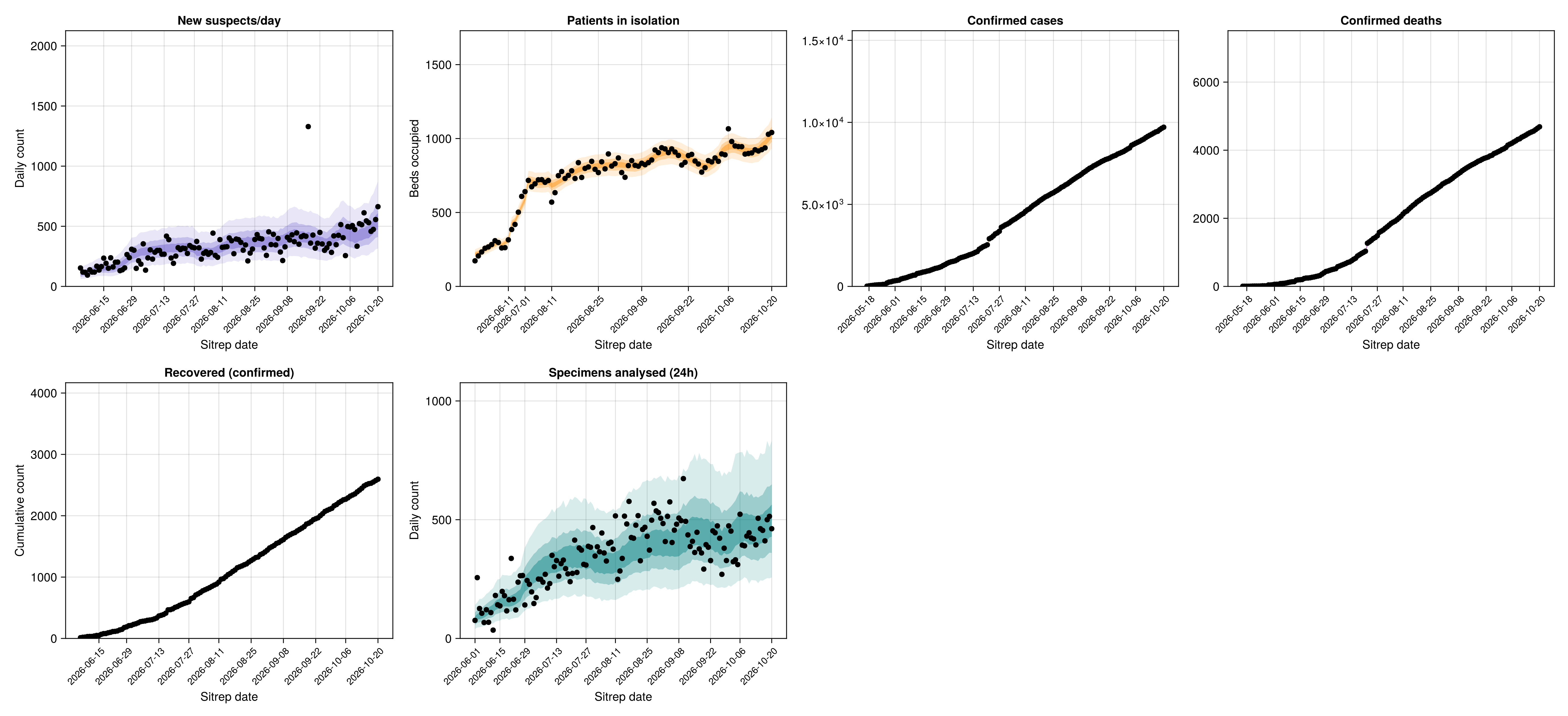
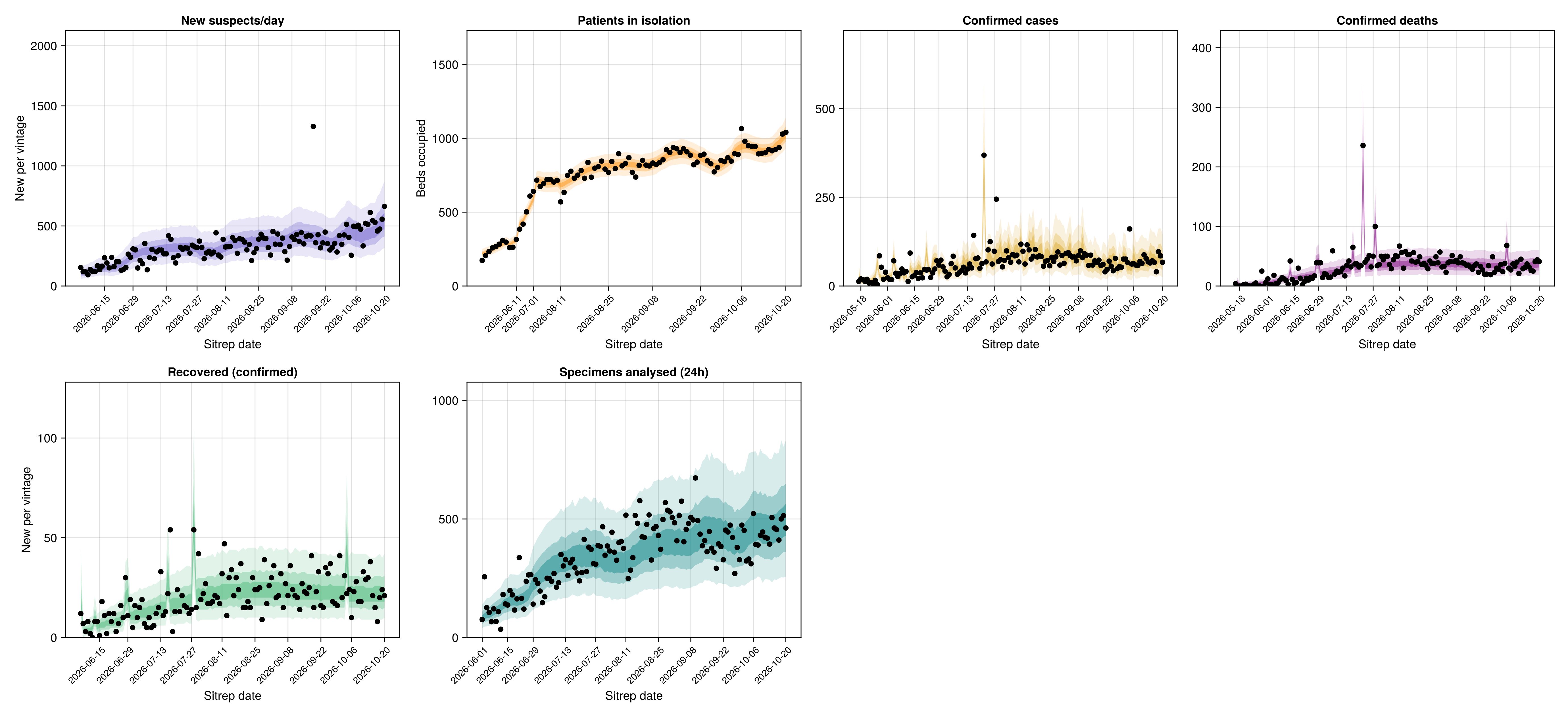
Per-vintage incidence
Whether the count reported between consecutive situation reports is reproduced.
Per-vintage incidence posterior predictive plot
joint_vintage_incidence_fig = plot_vintage_incidence_ppc(
    reporting_incidence_panels
);
Streams no longer reporting
Whether the streams that stopped before the cut-off are reproduced over the dates they cover.
Cumulative
Joint posterior predictive plot
joint_vintage_ppc_stopped_fig = plot_vintage_conditional_ppc(stopped_panels);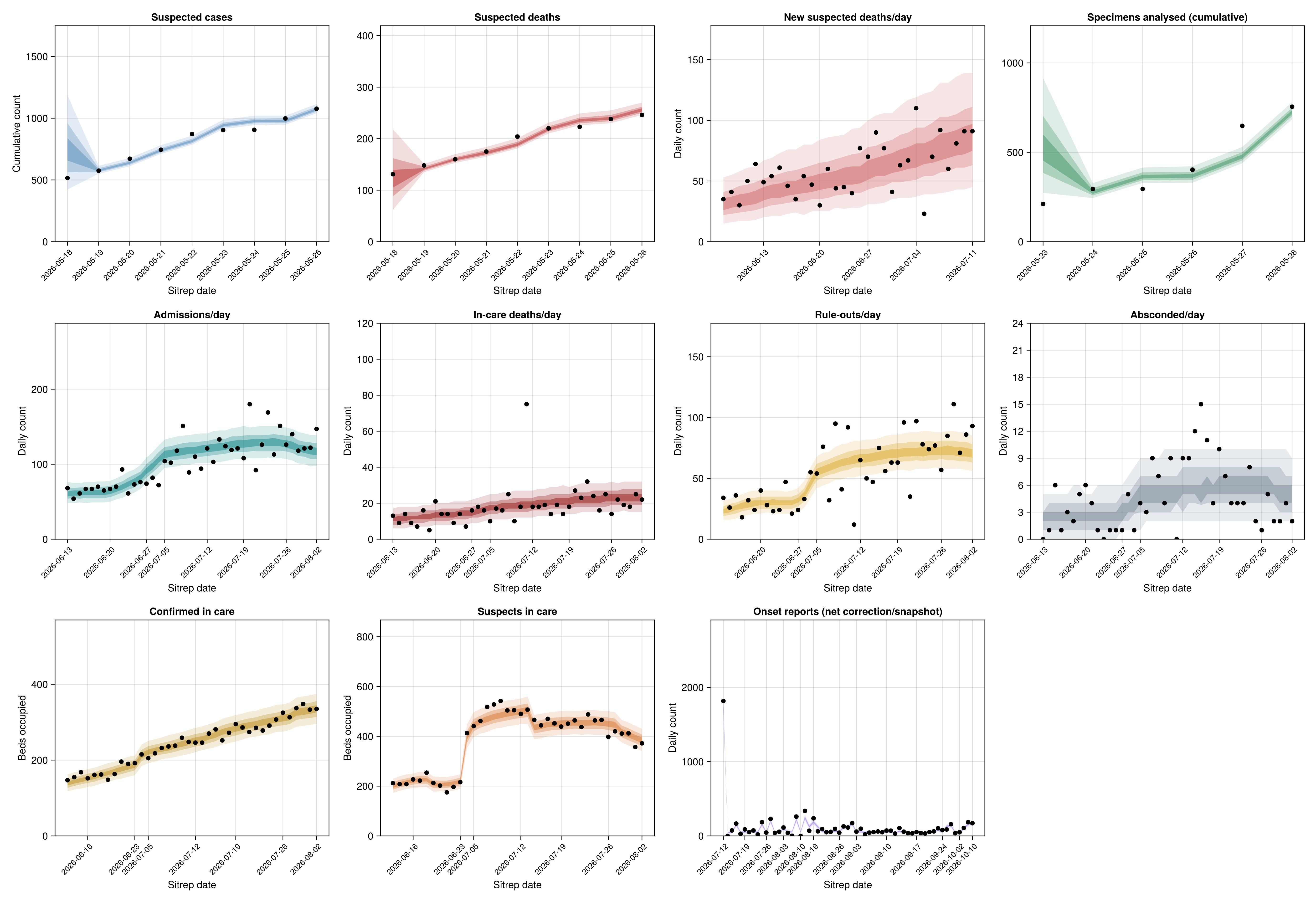
Per-vintage incidence
Per-vintage incidence posterior predictive plot
joint_vintage_incidence_stopped_fig = plot_vintage_incidence_ppc(
    stopped_incidence_panels
);
Stream calibration
Whether each stream's per-vintage predictions are calibrated against the observed counts.
stream_calibration_table = stream_calibration(vintage_panels);Per-stream calibration plot
stream_calibration_fig = plot_stream_calibration(stream_calibration_table);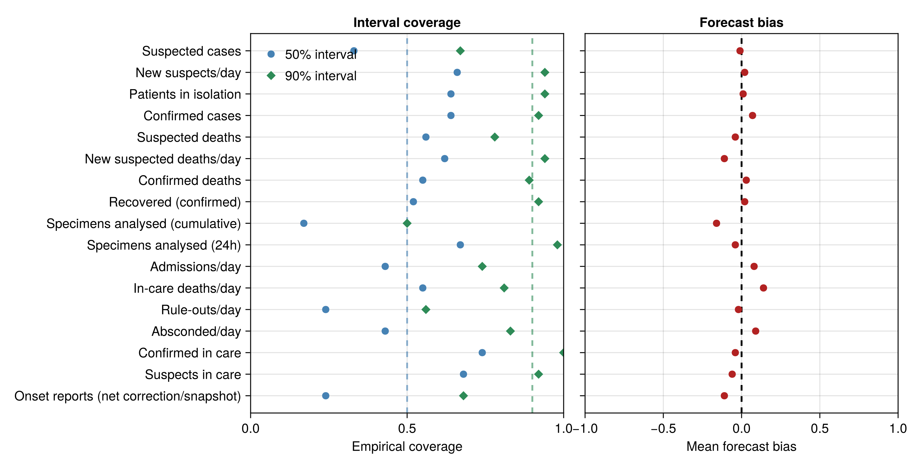
Per-stream calibration table
| Row | Stream | Vintages | Bias | 50% coverage | 90% coverage |
|---|---|---|---|---|---|
| String | Int64 | Float64 | Float64 | Float64 | |
| 1 | Suspected cases | 9 | -0.01 | 0.33 | 0.67 |
| 2 | New suspects/day | 129 | 0.02 | 0.66 | 0.94 |
| 3 | Patients in isolation | 90 | 0.01 | 0.64 | 0.94 |
| 4 | Confirmed cases | 149 | 0.07 | 0.64 | 0.92 |
| 5 | Suspected deaths | 9 | -0.04 | 0.56 | 0.78 |
| 6 | New suspected deaths/day | 32 | -0.11 | 0.62 | 0.94 |
| 7 | Confirmed deaths | 151 | 0.03 | 0.55 | 0.89 |
| 8 | Recovered (confirmed) | 130 | 0.02 | 0.52 | 0.92 |
| 9 | Specimens analysed (cumulative) | 6 | -0.16 | 0.17 | 0.5 |
| 10 | Specimens analysed (24h) | 132 | -0.04 | 0.67 | 0.98 |
| 11 | Admissions/day | 42 | 0.08 | 0.43 | 0.74 |
| 12 | In-care deaths/day | 42 | 0.14 | 0.55 | 0.81 |
| 13 | Rule-outs/day | 41 | -0.02 | 0.24 | 0.56 |
| 14 | Absconded/day | 42 | 0.09 | 0.43 | 0.83 |
| 15 | Confirmed in care | 38 | -0.04 | 0.74 | 1.0 |
| 16 | Suspects in care | 38 | -0.06 | 0.68 | 0.92 |
| 17 | Onset reports (net correction/snapshot) | 59 | -0.11 | 0.24 | 0.68 |
Exports
Whether the modelled Uganda export and export-death totals match the observed ones.
Scalar posterior predictive plot
# The dated counts are nested under their submodel prefix as a single
# per-day count vector `<prefix>.counts`; look it up by its VarName with
# `Prefixed` (matching the key by its `<obs>.counts` tail) so the
# deterministic `expected_*_T` quantities cannot be picked up by a loose
# substring, then sum each replicate's per-day vector into the total.
function _dated_total(pp, vn)
    return [sum(v) for v in vec(Array(pp[_Prefixed(vn)]))]
end;

pp_exports = _dated_total(pp_joint, @varname(export_obs.counts));
pp_exports_deaths = _dated_total(
    pp_joint, @varname(death_obs.counts)
);

joint_ppc_fig = plot_posterior_predictive(
    pp_exports, nothing,
    obs.exported_cases, nothing;
    pp_exports_deaths = pp_exports_deaths,
    obs_exports_deaths = obs.exports_deaths
);
Onset snapshot nowcasts
Whether the fitted reporting delay nowcasts each digitised onset snapshot to the latest figure covering its dates (see the symptom-onset reporting delay Methods section).
Nowcasts of the digitised reporting-triangle snapshots
# Each snapshot's own printed counts, read from the source blocks since the
# fitted stream holds only the corrections between snapshots.
_onset_readings = onset_snapshot_readings()
_onset_snap_by_day = Dict(
    obs.n - value(obs.cutoff - b.report_date) => b
        for b in _onset_readings.snaps
)
_onset_cells_by_report = Dict{Int, Vector{Int}}()
for (i, r) in enumerate(obs.onset_curve_history.report_days)
    push!(get!(_onset_cells_by_report, r, Int[]), i)
end
_onset_hazard = fitted_onset_hazard(fit_model("joint"), chn_joint)
_onset_daily_draws = onset_daily_draws(chn_joint)
_onset_replicated = onset_bar_replicator(
    chn_joint, Random.MersenneTwister(20260729)
)

# Each snapshot is nowcast to the delay of the figure each of its onset
# dates was last printed on, so the band and the latest reading are the
# same quantity.
_onset_panels = map(sort(collect(keys(_onset_cells_by_report)))) do R
    snap = _onset_snap_by_day[R]
    us = sort(obs.onset_curve_history.onset_days[_onset_cells_by_report[R]])
    observed = Float64[get(snap.onsets, grid_date(u), 0) for u in us]
    nowcast = onset_nowcast_draws(
        us, observed, [R - u for u in us],
        _onset_daily_draws, _onset_hazard; grid_start = _onset_grid_start,
        target_delays = [_onset_readings.last_report_day[u] - u for u in us]
    )
    (;
        title = string(snap.report_date), dates = grid_date.(us), observed,
        nowcast = [_onset_replicated(d) for d in nowcast],
        latest = [_onset_readings.last_printed[u] for u in us],
    )
end

onset_fit_fig = plot_onset_nowcast_grid(_onset_panels);
Onsets by date of onset
Reconstruct symptom onsets by date of onset
# The latest printed count for each onset date, from the snapshot
# readings above. The daily onset draws, the fitted hazard and the bar
# replicator are the ones the nowcasts use.
_onset_last_printed = _onset_readings.last_printed

# Ascertainment at onset day `u` for draw `i`, held flat at the ends of
# the fitted grid the same way the model extrapolates it.
function _onset_alpha(i::Integer, u::Integer)
    a = _onset_hazard.alpha[i]
    return a[clamp(u - _onset_grid_start + 1, 1, length(a))]
end

_onset_by_date_days = sort(collect(keys(_onset_last_printed)))

# Modelled onsets on each of those days, and the count the latest figure
# should print for them: the same onsets times the cumulative reported
# proportion at that figure's own delay, `_onset_grid_end - u`, so the
# band is a predictive for the bar actually plotted rather than for the
# eventual total. `onset_report_F` holds the calendar walk flat past its
# fitted support, which the most recent onset dates run into.
_onset_by_date_onsets = [
    [
        _onset_daily_draws[i][u]
            for i in eachindex(_onset_daily_draws)
    ]
        for u in _onset_by_date_days
]
_onset_by_date_printed = [
    [
        _onset_daily_draws[i][u] *
            onset_report_F(
            _onset_grid_end - u,
            _onset_hazard.logit_h0[i], _onset_hazard.γ[i],
            u, _onset_grid_start, _onset_alpha(i, u)
        )
            for i in eachindex(_onset_daily_draws)
    ]
        for u in _onset_by_date_days
]
# That count put through the measurement error of one digitised bar.
_onset_by_date_reps = [_onset_replicated(d) for d in _onset_by_date_printed]

onset_ppc_by_date_fig = let
    fig = CairoMakie.Figure(; size = (900, 380))
    ax = CairoMakie.Axis(
        fig[1, 1];
        title = "Symptom onsets by date of onset: modelled vs digitised",
        xlabel = "onset date", ylabel = "cases"
    )
    xs = Float64.(_onset_by_date_days)
    q(ds, p) = [quantile(d, p) for d in ds]
    CairoMakie.band!(
        ax, xs, q(_onset_by_date_onsets, 0.05),
        q(_onset_by_date_onsets, 0.95); color = (:seagreen, 0.2)
    )
    CairoMakie.lines!(
        ax, xs, q(_onset_by_date_onsets, 0.5);
        color = :seagreen, linewidth = 2
    )
    CairoMakie.band!(
        ax, xs, q(_onset_by_date_reps, 0.05),
        q(_onset_by_date_reps, 0.95); color = (:mediumpurple, 0.2)
    )
    CairoMakie.lines!(
        ax, xs, q(_onset_by_date_reps, 0.5);
        color = :mediumpurple, linewidth = 2
    )
    CairoMakie.scatter!(
        ax, xs,
        [_onset_last_printed[u] for u in _onset_by_date_days];
        color = :black, marker = :cross, markersize = 9
    )
    # Calendar labels on a grid-day axis, at weekly ticks so they do not
    # collide at this width.
    _ticks = _onset_by_date_days[1:7:end]
    ax.xticks = (Float64.(_ticks), string.(grid_date.(_ticks)))
    ax.xticklabelrotation = pi / 4
    CairoMakie.Legend(
        fig[2, 1],
        [
            CairoMakie.MarkerElement(color = :black, marker = :cross),
            CairoMakie.PolyElement(color = (:mediumpurple, 0.3)),
            CairoMakie.PolyElement(color = (:seagreen, 0.3)),
        ],
        [
            "digitised (latest)", "modelled posterior predictive",
            "modelled onsets",
        ];
        orientation = :horizontal, tellwidth = false, tellheight = true
    )
    fig
end;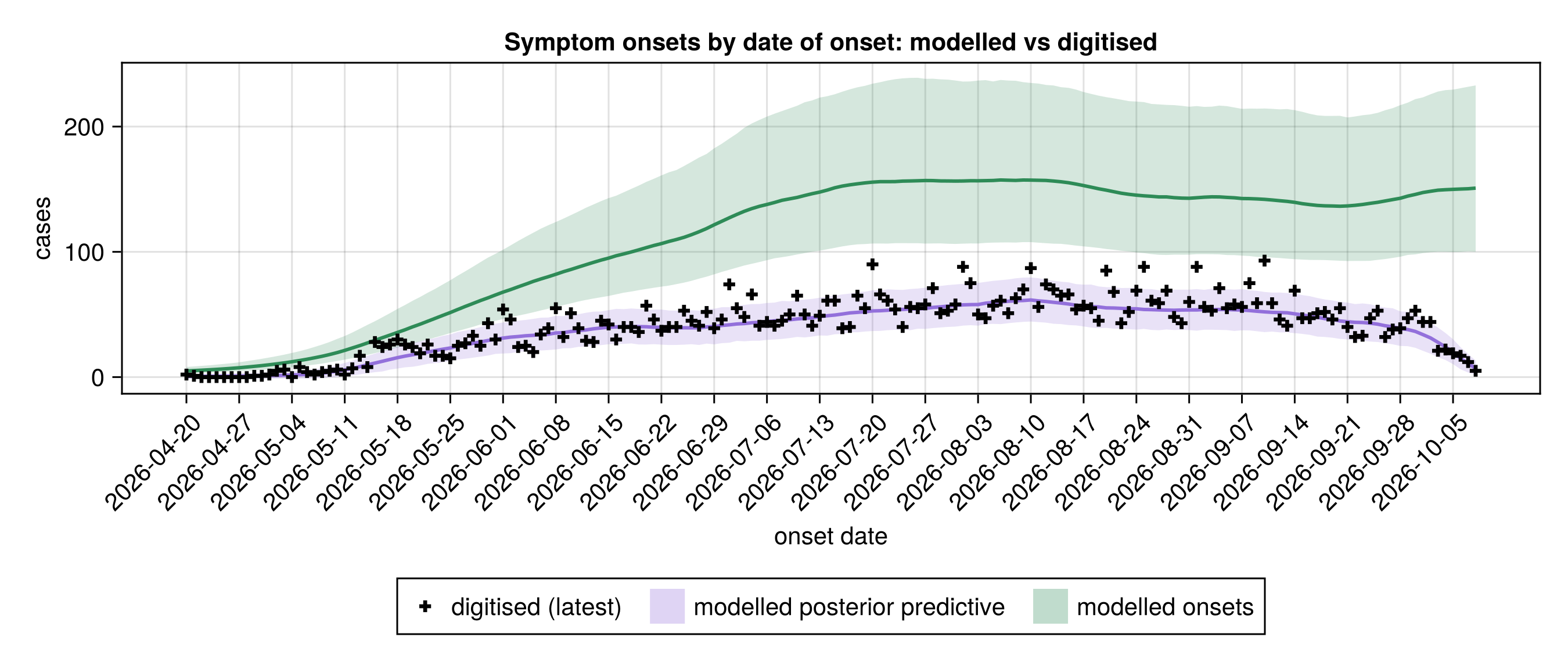
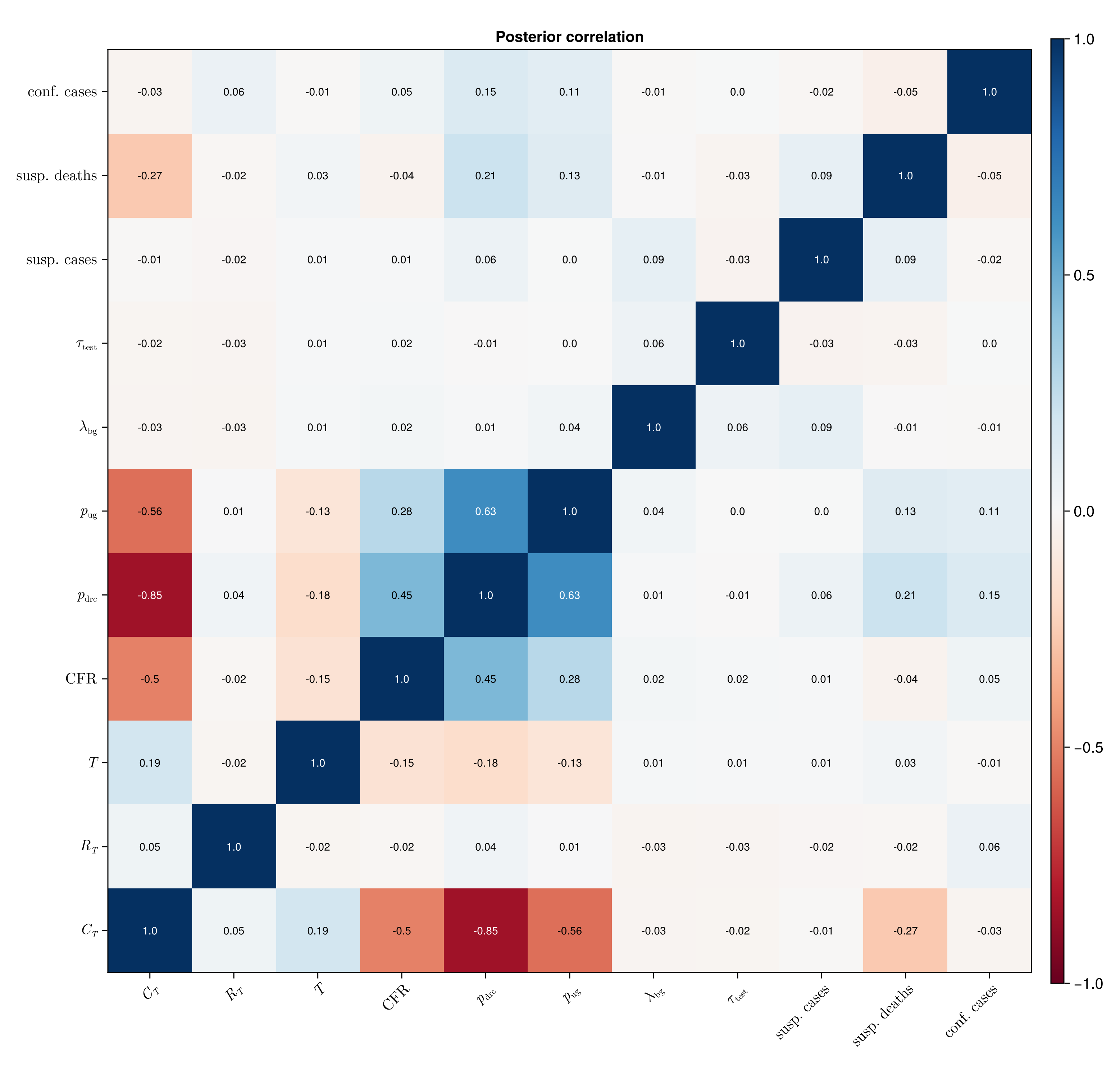
Posterior correlations and stream totals
Which headline quantities trade off against each other, and whether the stream totals match the observed ones.
Posterior correlation heatmap
correlation_fig = plot_correlation_heatmap(
    chn_joint,
    [
        :C_T, :R_T, :T, :CFR, :p_drc, :p_uganda, :lambda_bg, :tau_test,
        :expected_reports_T, :expected_deaths_T, :expected_confirmed_T,
    ];
    labels = Dict(
        :C_T => raw"C_T", :R_T => raw"R_T", :T => raw"T",
        :CFR => raw"\mathrm{CFR}", :p_drc => raw"p_\mathrm{drc}",
        :p_uganda => raw"p_\mathrm{ug}", :lambda_bg => raw"\lambda_\mathrm{bg}",
        :tau_test => raw"\tau_\mathrm{test}",
        :expected_reports_T => raw"\mathrm{susp.\ cases}",
        :expected_deaths_T => raw"\mathrm{susp.\ deaths}",
        :expected_confirmed_T => raw"\mathrm{conf.\ cases}"
    )
);
Stream totals against observed
# Per-draw modelled total of each stream, summed over its own reporting
# vintages (the confirmed total adds the unscored first-vintage baseline),
# reusing the posterior-predictive replicates built for the vintage panels.
_stream_total(reps) = [sum(Float64.(collect(r))) for r in vec(reps)]
_conf_baseline = isempty(obs.confirmed_history.counts) ? 0 :
    Int(obs.confirmed_history.counts[1])
stream_totals = (;
    suspected_cases = _stream_total(reported_panel.replicates),
    suspected_deaths = _stream_total(deaths_panel.replicates),
    confirmed_cases = _stream_total(confirmed_panel.replicates) .+ _conf_baseline,
    confirmed_deaths = _stream_total(confirmed_deaths_panel.replicates),
    analysed = _stream_total(tests_analysed_panel.replicates),
);
stream_observed = (;
    suspected_cases = Float64(obs.reported_history.counts[end]),
    suspected_deaths = Float64(obs.deaths_history.counts[end]),
    confirmed_cases = Float64(obs.confirmed_cases),
    confirmed_deaths = Float64(obs.confirmed_deaths_history.counts[end]),
    analysed = Float64(obs.lab_history.counts[end]),
);
stream_pairs_fig = plot_stream_pairs(stream_totals, stream_observed);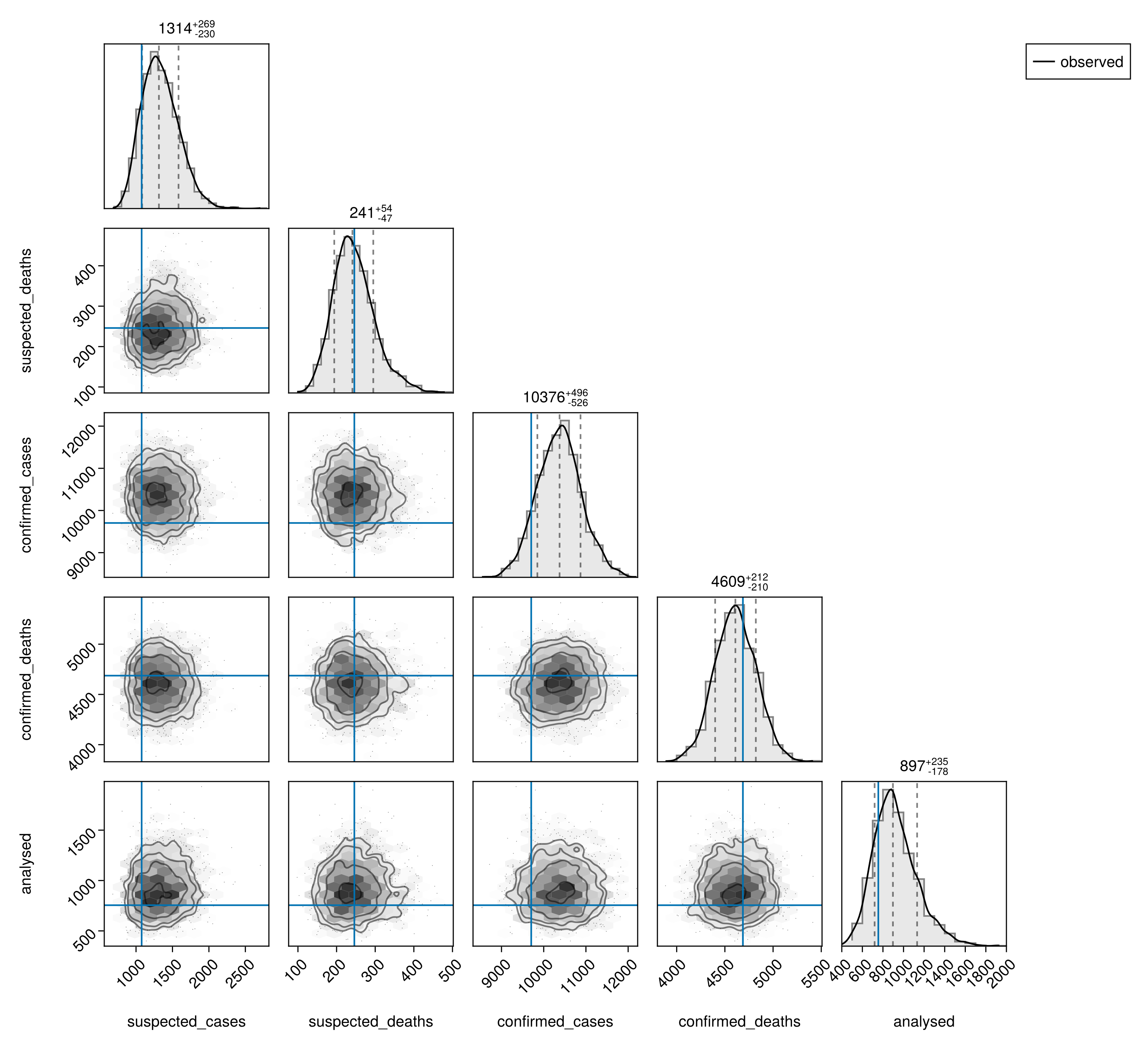
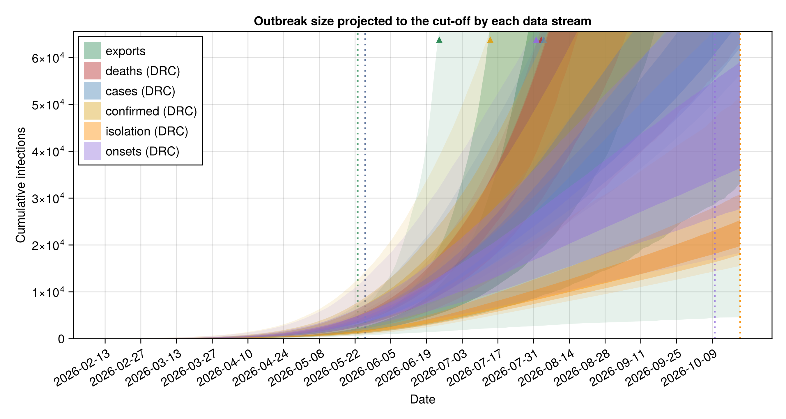
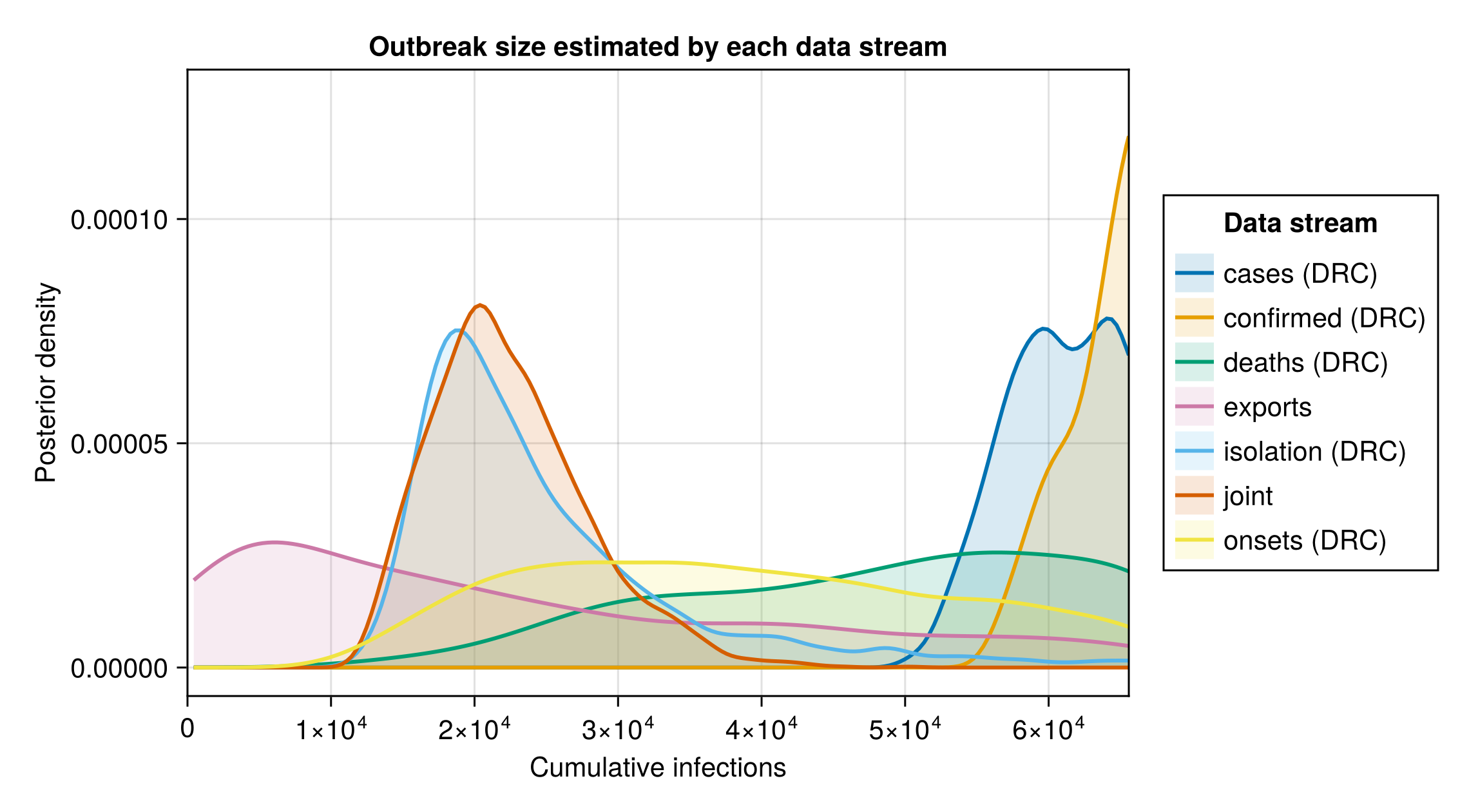
Outbreak size estimated by each data stream
Per-stream infection-count table
streams_C_table = streams_table(
    "exports" => posterior_C_exports,
    "deaths (DRC)" => posterior_C_deaths,
    "cases (DRC)" => posterior_C_cases,
    "confirmed (DRC)" => posterior_C_confirmed,
    "isolation (DRC)" => posterior_C_treatment,
    "onsets (DRC)" => posterior_C_onsets,
    "joint" => posterior_C_joint
);| Stream | Lower 90% | Lower 60% | Lower 30% | Upper 30% | Upper 60% | Upper 90% |
|---|---|---|---|---|---|---|
| exports | 4570 | 33179 | 157329 | 3660727 | 17368992 | 27610370 |
| deaths (DRC) | 63222 | 165324 | 400409 | 412256 | 433924 | 1579105 |
| cases (DRC) | 56441 | 62140 | 67766 | 85810 | 106359 | 174586 |
| confirmed (DRC) | 71605 | 84383 | 95937 | 127853 | 155831 | 251407 |
| isolation (DRC) | 15534 | 17937 | 19773 | 25332 | 30853 | 51376 |
| onsets (DRC) | 18338 | 27695 | 36410 | 59253 | 81863 | 148788 |
| joint | 14896 | 17752 | 19852 | 23821 | 26643 | 32793 |
Per-stream projected-trajectory plot
# Per-draw cumulative-infection trajectory carried by each single-stream
# fit out to the cut-off on day `n`, so streams whose data ends earlier are
# still projected to today.
function _cuminf(chn)
    mat = chn[:cumulative_infections]
    return [collect(v) for v in vec(collect(mat))]
end
# Grid day a stream's data last reports, used for the dotted rule. The
# suspected case and death histories freeze at 26 May; exports and confirmed
# run to the cut-off.
_last_day(days) = isempty(days) ? nothing : maximum(days)

stream_traj_fig = plot_stream_trajectories(
    [
        (;
            label = "exports", trajs = _cuminf(chn_exports),
            last_day = _last_day(
                vcat(
                    obs.export_case_days,
                    obs.export_death_days
                )
            ), colour = :seagreen,
        ),
        (;
            label = "deaths (DRC)", trajs = _cuminf(chn_deaths),
            last_day = _last_day(obs.deaths_history.days),
            colour = :firebrick,
        ),
        (;
            label = "cases (DRC)", trajs = _cuminf(chn_cases),
            last_day = _last_day(obs.reported_history.days),
            colour = :steelblue,
        ),
        (;
            label = "confirmed (DRC)", trajs = _cuminf(chn_confirmed),
            last_day = _last_day(obs.confirmed_history.days),
            colour = :goldenrod,
        ),
        (;
            label = "isolation (DRC)", trajs = _cuminf(chn_treatment),
            last_day = _last_day(obs.isolation_history.days),
            colour = :darkorange,
        ),
        (;
            label = "onsets (DRC)", trajs = _cuminf(chn_onsets),
            last_day = _last_day(obs.onset_curve_history.report_days),
            colour = :mediumpurple,
        ),
    ];
    n = obs.n, seeding = obs.seeding,
    # Twice the joint fit's 90% upper, the crop the cut-off density figure
    # below already uses. The exports-only fit bounds the infection count
    # so weakly that its 90% upper reaches the source population, which on
    # a free axis puts every other stream on the baseline.
    ymax = 2.0 * quantile(posterior_C_joint, 0.95)
);
Cut-off infection-count density plot
# Scale the x-axis to twice the joint-fit 90% upper bound, so the joint and
# the streams that track it read clearly while the confirmed-only tail runs
# off the axis rather than dominating it.
density_xmax = 2.0 * quantile(posterior_C_joint, 0.95)

cumulative_density_fig = plot_cumulative_cases(
    "exports" => posterior_C_exports,
    "deaths (DRC)" => posterior_C_deaths,
    "cases (DRC)" => posterior_C_cases,
    "confirmed (DRC)" => posterior_C_confirmed,
    "isolation (DRC)" => posterior_C_treatment,
    "onsets (DRC)" => posterior_C_onsets,
    "joint" => posterior_C_joint;
    scenarios = [], xmax = density_xmax
);
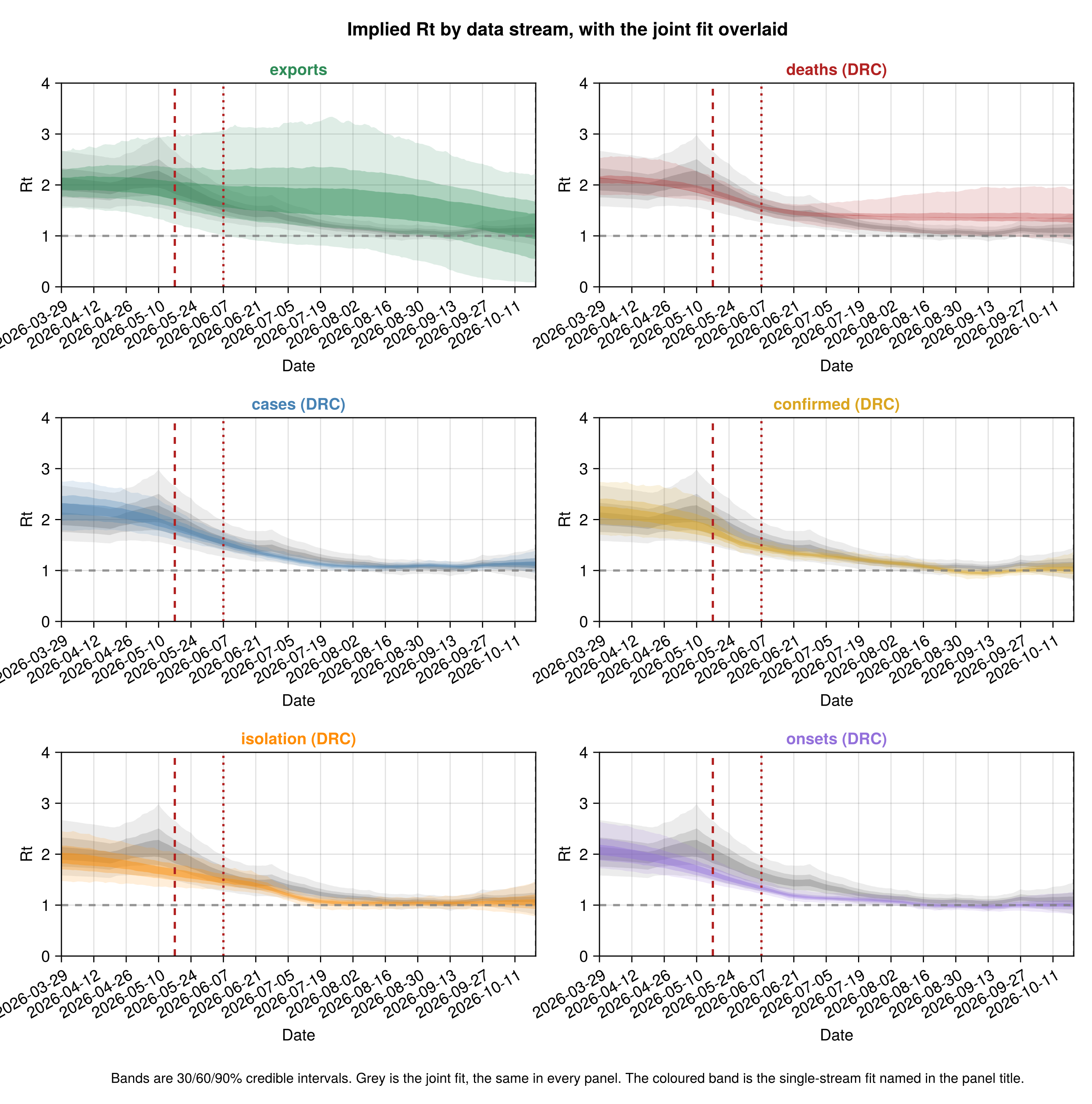
Reproduction number estimated by each data stream
Per-stream implied-Rt plot
# The per-stream fits walk Rt from day 1 (the default `rt_start`), while the
# joint walks from `RT_WALK_LEAD` days before the first situation report; the
# shared `display_start` is the joint renewal start so every stream reads over
# the same established window. `ramp` matches the joint Rt figure.
_rt_walk_start_joint = clamp(_BREAKPOINT - RT_WALK_LEAD, _rt_start_plot, obs.n);
stream_rt_fig = plot_rt_streams(
    [
        (;
            label = "exports", chn = chn_exports, rt_start = 1,
            rt_walk_start = 1, colour = :seagreen,
        ),
        (;
            label = "deaths (DRC)", chn = chn_deaths, rt_start = 1,
            rt_walk_start = 1, colour = :firebrick,
        ),
        (;
            label = "cases (DRC)", chn = chn_cases, rt_start = 1,
            rt_walk_start = 1, colour = :steelblue,
        ),
        (;
            label = "confirmed (DRC)", chn = chn_confirmed, rt_start = 1,
            rt_walk_start = 1, colour = :goldenrod,
        ),
        (;
            label = "isolation (DRC)", chn = chn_treatment, rt_start = 1,
            rt_walk_start = 1, colour = :darkorange,
        ),
        (;
            label = "onsets (DRC)", chn = chn_onsets, rt_start = 1,
            rt_walk_start = 1, colour = :mediumpurple,
        ),
    ];
    joint = (;
        label = "joint", chn = chn_joint, rt_start = _rt_start_plot,
        rt_walk_start = _rt_walk_start_joint,
    ),
    n = obs.n, breakpoint = _BREAKPOINT,
    as_of_date = string(obs.cutoff), seeding = obs.seeding,
    display_start = _rt_start_plot, ramp = RT_INTERVENTION_RAMP
);
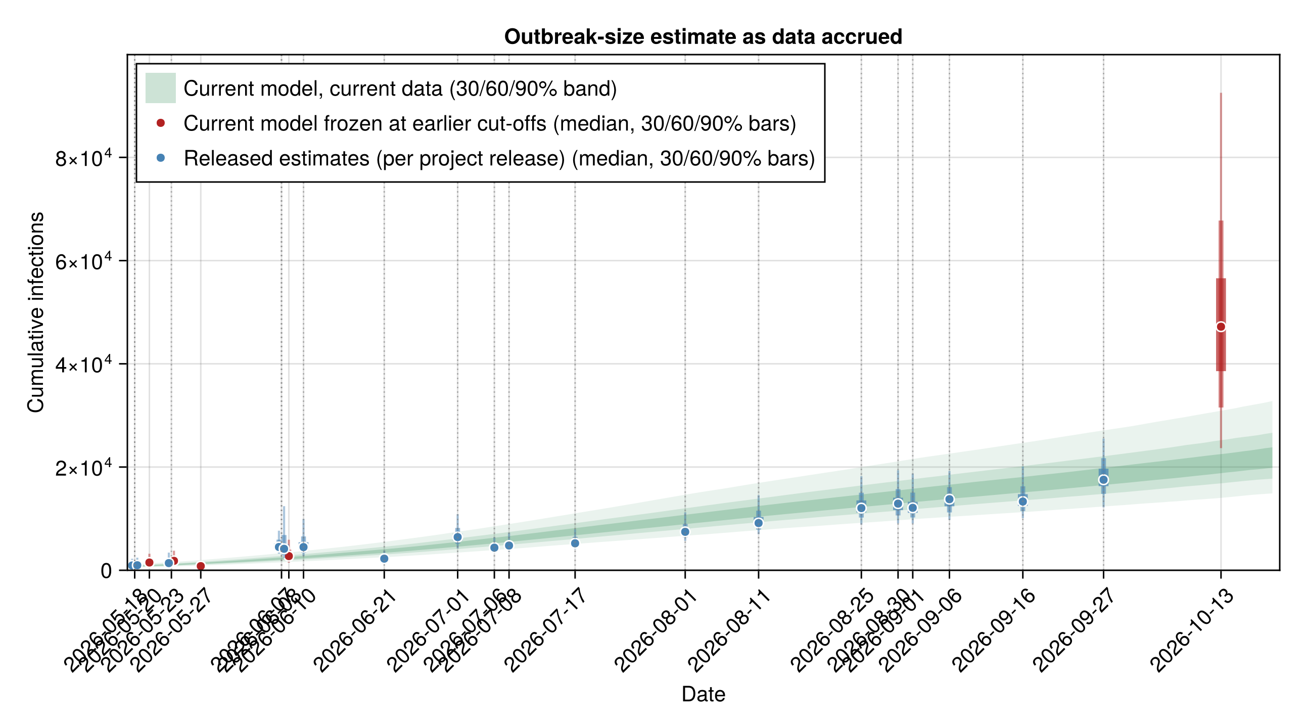
Estimate evolution across releases
How the outbreak-size estimate has moved as situation reports accrued.
Released estimates and the current-model frozen re-fits
# Released median and 30/60/90% intervals per release, from
# `data/released_estimates.csv`. Each tuple is
# `(date, median, lo30, hi30, lo60, hi60, lo90, hi90)`.
release_evolution = [
    (
        string(r.date), r.median, r.lo30, r.hi30, r.lo60, r.hi60,
        r.lo90, r.hi90,
    ) for r in eachrow(released_df)
]

# The current model frozen at earlier cut-offs, each its own discrete
# estimate: the McCabe-matched cut-offs (20, 23, 27 May), the 8 June Chamla
# confirmed-case anchor and the one-week-back validation fit
# (`frozen_lastweek`, at `validation_cutoff`). Each tuple carries the
# median and 30/60/90% credible bounds from the frozen draws; `round_fn`
# rounds to a whole count for outbreak size, and is passed through
# unrounded for a continuous quantity such as R0.
function _ci369(xs; round_fn = x -> round(Int, x))
    q(p) = round_fn(quantile(xs, p))
    return (q(0.5), q(0.35), q(0.65), q(0.2), q(0.8), q(0.05), q(0.95))
end
frozen_by_cutoff[validation_cutoff] = frozen_lastweek
# The cut-offs every frozen fit above was made at, shared by the
# outbreak-size and R0 by-release overlays below.
_frozen_matched_cutoffs = sort(
    union(
        frozen_cutoffs,
        [validation_cutoff, default_chamla_cutoff()]
    )
)
frozen_matched = [(c, _ci369(frozen_C(c))...) for c in _frozen_matched_cutoffs]

# The current-data, current-model estimate as the cumulative-infection
# trajectory over the day grid (one calendar date per grid day, day 1 is
# the seeding date), summarised by per-day 30/60/90% credible bounds. This
# is the same latent quantity the cumulative-trajectory figure shows, so
# the current estimate rises over time on the release-date axis instead of
# sitting flat. Drawn against calendar dates, it lines up with the
# release and frozen points.
infection_trajectory = let
    mat = chn_joint[:cumulative_infections]
    trajs = [collect(v) for v in vec(collect(mat))]
    # Only over the comparison window — from the earliest release date to the
    # cut-off — not back to the seeding date.
    start_day = obs.n - value(obs.cutoff - Date(release_evolution[1][1]))
    days = max(start_day, 1):obs.n
    dates = [obs.seeding + Day(d - 1) for d in days]
    q(d, p) = quantile(Float64[t[d] for t in trajs], p)
    (
        dates,
        [q(d, 0.35) for d in days], [q(d, 0.65) for d in days],
        [q(d, 0.2) for d in days], [q(d, 0.8) for d in days],
        [q(d, 0.05) for d in days], [q(d, 0.95) for d in days],
    )
end

evolution_fig = plot_estimate_evolution(
    release_evolution;
    renewal = frozen_matched,
    renewal_label = "Current model frozen at earlier cut-offs",
    trajectory = infection_trajectory,
    title = "Outbreak-size estimate as data accrued"
);
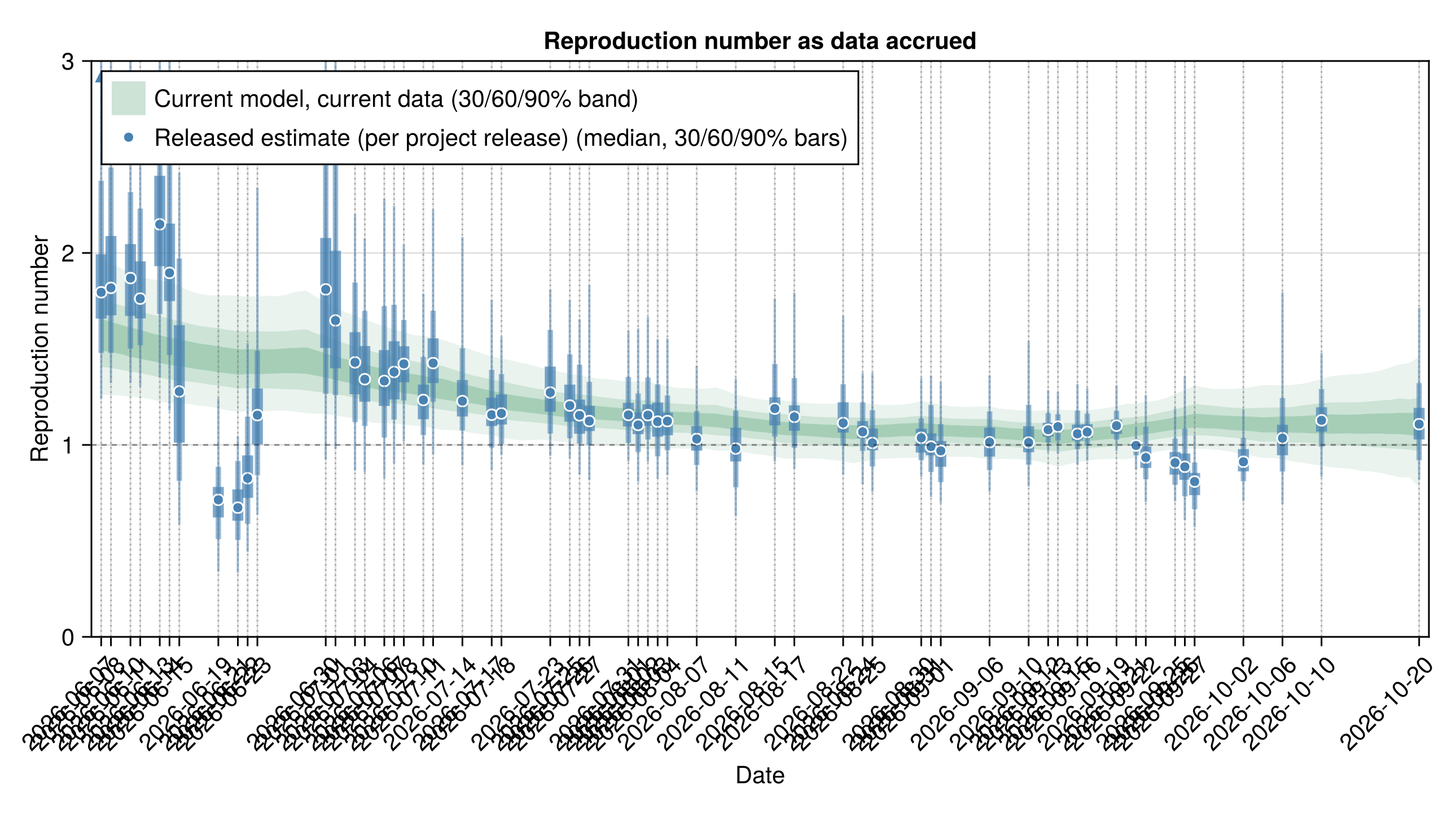
Reproduction number by release
Reproduction number per release with the current-fit band
rt_release_df = CSV.read(
    joinpath(pkgdir(BVDOutbreakSize), "data", "rt_by_release.csv"), DataFrame
)
rt_release = [
    (
        string(r.date), r.median, r.lo30, r.hi30, r.lo60, r.hi60,
        r.lo90, r.hi90,
    ) for r in eachrow(rt_release_df)
]

# The current fit's daily Rt over its established window, summarised per day
# into a 30/60/90% band, reusing the same walk reconstruction the Rt figure
# uses so the band lines up with the per-release points on the calendar axis.
# The band is drawn only from the first release date onward, so it spans the
# same window as the per-release estimates rather than extending back to the
# renewal start. The first release day is the earliest date in
# `rt_by_release.csv` as a grid day; the walk is still reconstructed from the
# renewal start `_rt_start_plot` (the model knot grid) and the window is
# clamped into the reconstructed range so the quantiles never hit masked days.
rt_release_trajectory = let
    rt_walk_start = clamp(_BREAKPOINT - RT_WALK_LEAD, _rt_start_plot, obs.n)
    mat = reconstruct_rt(
        chn_joint; n = obs.n, breakpoint = _BREAKPOINT,
        rt_start = _rt_start_plot, rt_walk_start = rt_walk_start,
        ramp = RT_INTERVENTION_RAMP
    )
    first_release_day = clamp(
        value(minimum(rt_release_df.date) - obs.seeding) + 1,
        _rt_start_plot, obs.n
    )
    days = first_release_day:obs.n
    dates = [obs.seeding + Day(d - 1) for d in days]
    q(d, p) = quantile(collect(skipmissing(@view mat[:, d])), p)
    (
        dates,
        [q(d, 0.35) for d in days], [q(d, 0.65) for d in days],
        [q(d, 0.2) for d in days], [q(d, 0.8) for d in days],
        [q(d, 0.05) for d in days], [q(d, 0.95) for d in days],
    )
end

# One fixed reproduction-number axis across both figures below. The
# estimates sit around one and the widest stream's 90% upper pulls a free
# axis past four, which flattens every panel onto the lower quarter of its
# range. An interval past the crop is clamped and marked, so nothing is
# silently cut. The basic reproduction number keeps its own axis: it sits
# around two with tails near four, and the same crop would clip the
# estimates themselves.
const _RT_AXIS_MAX = 3.0

rt_evolution_fig = plot_estimate_evolution(
    rt_release;
    trajectory = rt_release_trajectory,
    ylabel = "Reproduction number",
    title = "Reproduction number as data accrued",
    released_label = "Released estimate (per project release)",
    trajectory_label = "Current model, current data",
    refline = 1.0,
    ymax = _RT_AXIS_MAX
);
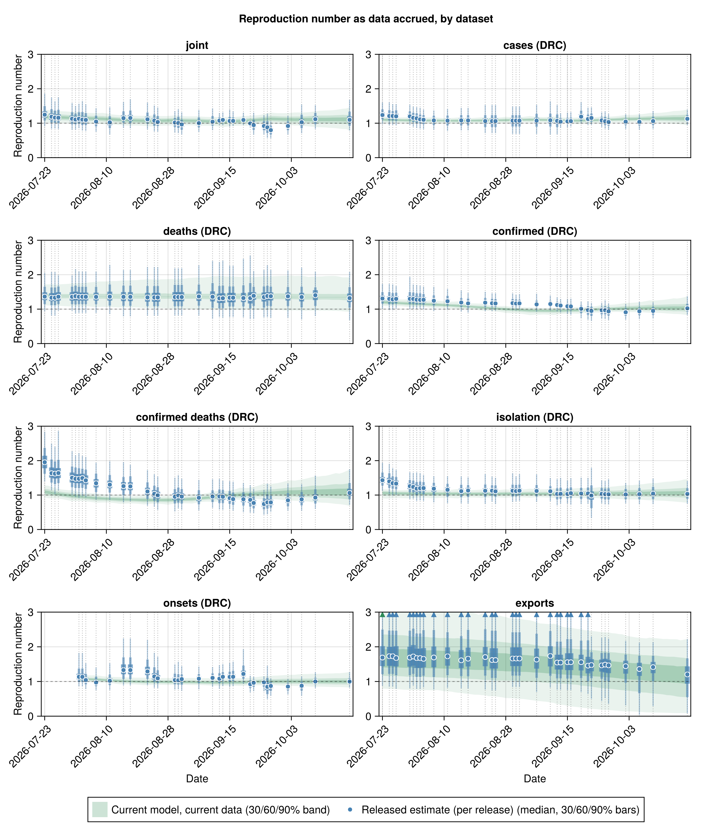
Reproduction number by release and dataset
Reproduction number per release by fit
# Schema of the per-release, per-fit estimate tables written by
# scripts/score_releases.jl from each release's stream_estimates.csv.
_by_stream_schema = (;
    release = String, date = Date, fit = String,
    median = Float64, lo30 = Float64, hi30 = Float64, lo60 = Float64,
    hi60 = Float64, lo90 = Float64, hi90 = Float64,
)

# Fits in a fixed order, the joint first, so the panels do not reshuffle
# between builds. Labels match the per-stream table above.
# Recovered is absent because it has no individual fit.
_fit_order = [
    "joint", "cases", "deaths", "confirmed", "confirmed_deaths",
    "treatment", "onsets", "exports",
]
_fit_labels = Dict(
    "joint" => "joint", "cases" => "cases (DRC)",
    "deaths" => "deaths (DRC)", "confirmed" => "confirmed (DRC)",
    "confirmed_deaths" => "confirmed deaths (DRC)",
    "treatment" => "isolation (DRC)", "onsets" => "onsets (DRC)",
    "exports" => "exports"
)

# Group a per-fit estimate table into the label => tuples pairs the faceted
# plot takes, keyed on the date so the mixed release tag shapes
# (`results-v1.9.0` and `results-1243`) never reach the axis.
function _fit_groups(df)
    return [
        get(_fit_labels, f, f) =>
            [
            (
                string(r.date), r.median, r.lo30, r.hi30, r.lo60, r.hi60,
                r.lo90, r.hi90,
            ) for r in eachrow(df) if r.fit == f
        ]
            for f in _fit_order
    ]
end

# Per-fit reproduction-number trajectory, reconstructing the walk exactly as
# `plot_rt_streams` does per stream.
function _stream_rt_trajectory(chn, dates; rt_start, rt_walk_start)
    mat = reconstruct_rt(
        chn; n = obs.n, breakpoint = _BREAKPOINT,
        rt_start = rt_start, rt_walk_start = rt_walk_start,
        ramp = RT_INTERVENTION_RAMP
    )
    first_date = isempty(dates) ? obs.seeding : minimum(dates)
    first_day = clamp(value(first_date - obs.seeding) + 1, rt_start, obs.n)
    days = first_day:obs.n
    ds = [obs.seeding + Day(d - 1) for d in days]
    q(d, p) = quantile(collect(skipmissing(@view mat[:, d])), p)
    return (
        ds,
        [q(d, 0.35) for d in days], [q(d, 0.65) for d in days],
        [q(d, 0.2) for d in days], [q(d, 0.8) for d in days],
        [q(d, 0.05) for d in days], [q(d, 0.95) for d in days],
    )
end

# The single-stream chains and their renewal-walk starts, keyed on the fit
# id the per-release tables use. Both the joint walk start and the day-1
# per-stream starts are the ones the per-stream implied-Rt figure above
# uses, so the bands here match it. Confirmed deaths has no trajectory
# here: its panel still draws its release points alone.
_stream_chains = (
    "joint" => (;
        chn = chn_joint, rt_start = _rt_start_plot,
        rt_walk_start = _rt_walk_start_joint,
    ),
    "cases" => (; chn = chn_cases, rt_start = 1, rt_walk_start = 1),
    "deaths" => (; chn = chn_deaths, rt_start = 1, rt_walk_start = 1),
    "confirmed" => (; chn = chn_confirmed, rt_start = 1, rt_walk_start = 1),
    "confirmed_deaths" => (;
        chn = chn_confirmed_deaths, rt_start = 1,
        rt_walk_start = 1,
    ),
    "treatment" => (; chn = chn_treatment, rt_start = 1, rt_walk_start = 1),
    "onsets" => (; chn = chn_onsets, rt_start = 1, rt_walk_start = 1),
    "exports" => (; chn = chn_exports, rt_start = 1, rt_walk_start = 1),
)

# Build a fit label => trajectory dictionary from a per-release table,
# restricted to the fits `_stream_chains` names. A fit with no row in `df`
# gets no trajectory, so its panel still draws its release points alone.
function _rt_trajectories(df)
    trajs = Dict{String, Any}()
    for (fid, cfg) in _stream_chains
        fdates = df.date[df.fit .== fid]
        isempty(fdates) && continue
        trajs[get(_fit_labels, fid, fid)] = _stream_rt_trajectory(
            cfg.chn, fdates; rt_start = cfg.rt_start,
            rt_walk_start = cfg.rt_walk_start
        )
    end
    return trajs
end

rt_stream_df = _release_data(
    "rt_by_release_by_stream.csv",
    _by_stream_schema
)
rt_stream_fig = plot_evolution_by_group(
    _fit_groups(rt_stream_df);
    trajectories = _rt_trajectories(rt_stream_df),
    ylabel = "Reproduction number",
    title = "Reproduction number as data accrued, by dataset",
    released_label = "Released estimate (per release)",
    refline = 1.0,
    ymax = _RT_AXIS_MAX,
    empty_note = "No per-dataset reproduction numbers saved yet."
);
Basic reproduction number by release
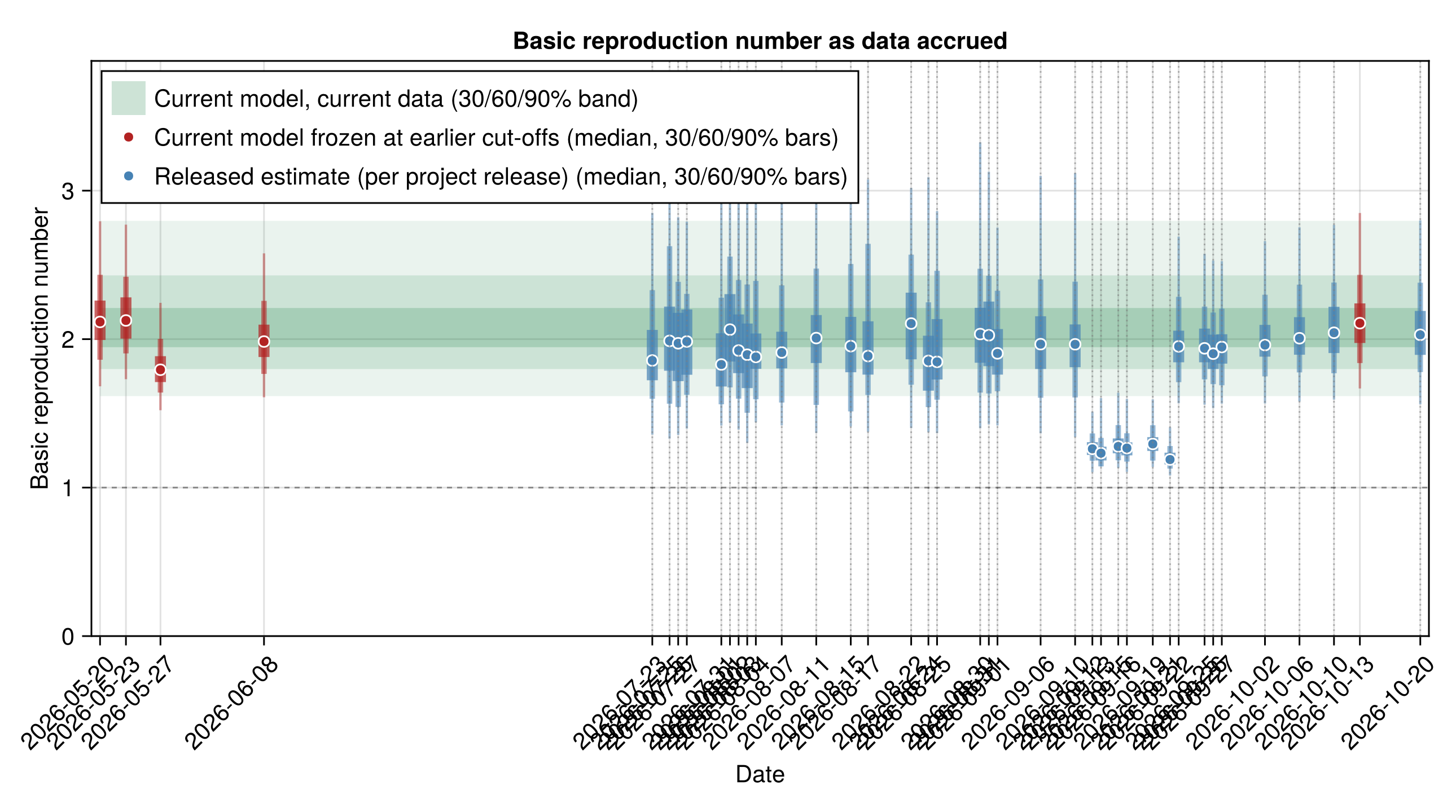
Basic reproduction number per release with frozen re-fits and the current-fit band
# Per-release R0 points from r0_by_release.csv, read through the typed
# fallback so a missing or header-only file (until a release carries
# `rt_state.log_R0` in its posterior draws) does not break the build. The
# schema mirrors rt_by_release.csv.
_r0_schema = (;
    release = String, date = Date, median = Float64,
    lo30 = Float64, hi30 = Float64, lo60 = Float64, hi60 = Float64,
    lo90 = Float64, hi90 = Float64,
)
r0_release_df = _release_data("r0_by_release.csv", _r0_schema)
r0_release = [
    (
        string(r.date), r.median, r.lo30, r.hi30, r.lo60, r.hi60,
        r.lo90, r.hi90,
    ) for r in eachrow(r0_release_df)
]

# The current model frozen at earlier cut-offs, one discrete estimate per
# cut-off, reusing the same frozen fits `frozen_matched` above already
# computed. No extra fits are run. Each tuple carries the median and
# 30/60/90% credible bounds of that frozen fit's own R0 draws, unrounded
# since R0 is continuous.
frozen_r0_matched = [
    (c, _ci369(frozen_R0(c); round_fn = identity)...)
        for c in _frozen_matched_cutoffs
]

# The current fit's R0 posterior is a single distribution rather than a
# daily series, so it summarises into a flat 30/60/90% reference band. The
# window runs from the earliest mark on the axis, the first frozen cut-off
# or release point, to the current cut-off, so the band reads behind both
# series rather than only their recent end.
r0_reference = let
    draws = r0_walk_draws(chn_joint)
    q(p) = quantile(draws, p)
    first_date = min(
        minimum(Date.(_frozen_matched_cutoffs)),
        isempty(r0_release_df.date) ? obs.cutoff :
            minimum(r0_release_df.date)
    )
    dates = [first_date, obs.cutoff]
    (
        dates, fill(q(0.35), 2), fill(q(0.65), 2), fill(q(0.2), 2),
        fill(q(0.8), 2), fill(q(0.05), 2), fill(q(0.95), 2),
    )
end

r0_evolution_fig = plot_estimate_evolution(
    r0_release;
    renewal = frozen_r0_matched,
    renewal_label = "Current model frozen at earlier cut-offs",
    trajectory = r0_reference,
    ylabel = "Basic reproduction number",
    title = "Basic reproduction number as data accrued",
    released_label = "Released estimate (per project release)",
    trajectory_label = "Current model, current data",
    refline = 1.0
);
Basic reproduction number by release and dataset
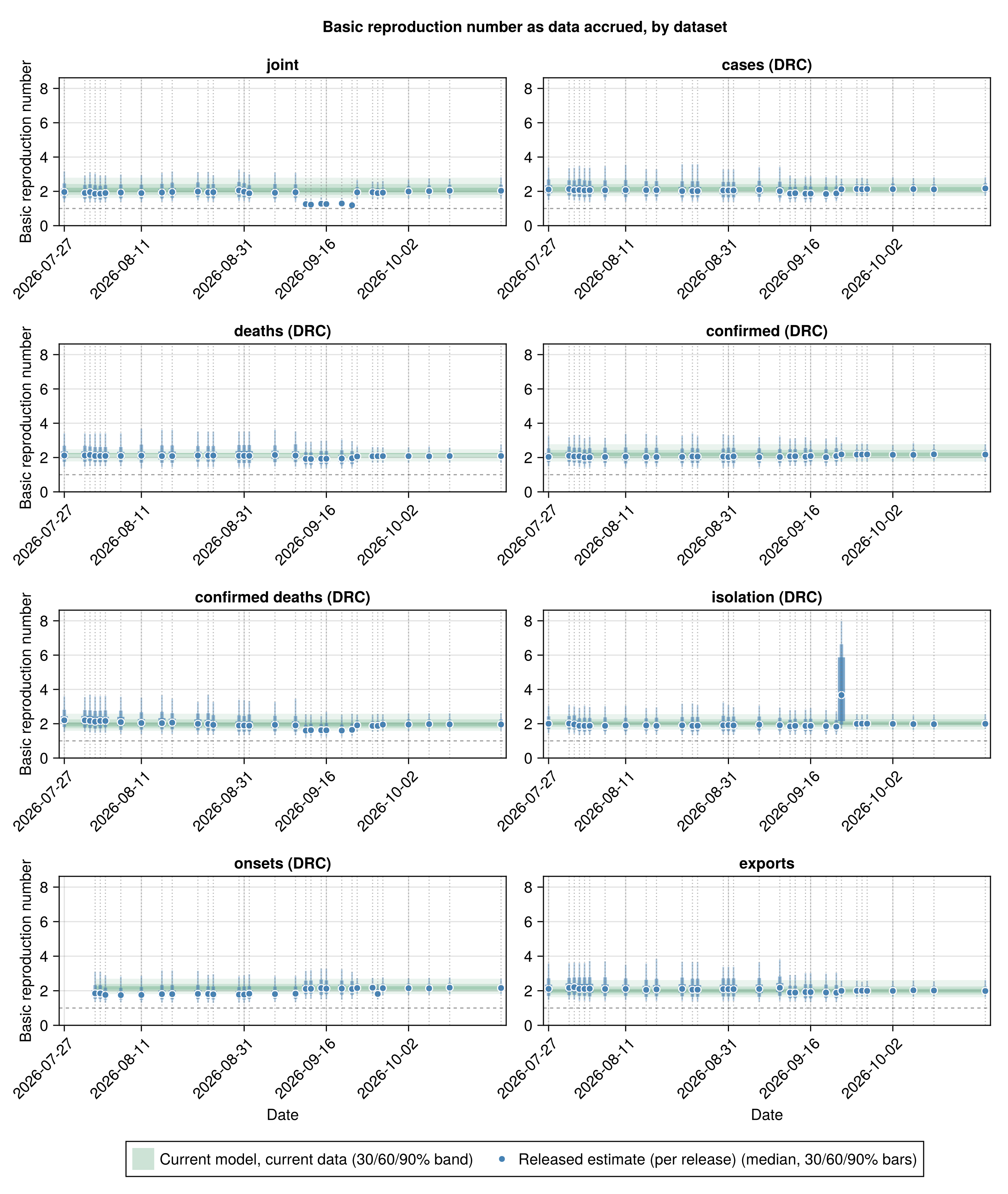
Basic reproduction number per release by fit
# Per-fit R0 flat reference band, the by-dataset counterpart of
# `r0_reference` above, a single distribution rather than a daily walk, so
# each fit's band is flat across its own release window. `r0_walk_draws`
# probes for the walk base, so a single-stream model built without its own
# renewal walk drops its band instead of erroring.
function _r0_stream_trajectory(chn, dates)
    draws = r0_walk_draws(chn)
    isnothing(draws) && return nothing
    q(p) = quantile(draws, p)
    first_date = isempty(dates) ? obs.seeding : minimum(dates)
    ds = [first_date, obs.cutoff]
    return (
        ds, fill(q(0.35), 2), fill(q(0.65), 2), fill(q(0.2), 2),
        fill(q(0.8), 2), fill(q(0.05), 2), fill(q(0.95), 2),
    )
end

# Build a fit label => trajectory dictionary from a per-release R0 table,
# restricted to the fits `_stream_chains` names, the same restriction the
# reproduction-number-by-dataset trajectories use. A fit with no row in
# `df`, or whose chain carries no walk base, gets no trajectory, so its
# panel still draws its release points alone.
function _r0_trajectories(df)
    trajs = Dict{String, Any}()
    for (fid, cfg) in _stream_chains
        fdates = df.date[df.fit .== fid]
        isempty(fdates) && continue
        traj = _r0_stream_trajectory(cfg.chn, fdates)
        isnothing(traj) || (trajs[get(_fit_labels, fid, fid)] = traj)
    end
    return trajs
end

r0_stream_df = _release_data(
    "r0_by_release_by_stream.csv",
    _by_stream_schema
)
r0_stream_fig = plot_evolution_by_group(
    _fit_groups(r0_stream_df);
    trajectories = _r0_trajectories(r0_stream_df),
    ylabel = "Basic reproduction number",
    title = "Basic reproduction number as data accrued, by dataset",
    released_label = "Released estimate (per release)",
    refline = 1.0,
    empty_note = "No per-dataset basic reproduction numbers saved yet."
);
Sensitivity to assumptions
The joint model re-fitted with one assumption changed at a time.
Delay sensitivity
The death stream dates the outbreak from how far deaths lag symptom onset, so the assumed onset-to-death delay sets the implied infection count. The baseline uses the hospital-pathway delay from the Isiro 2012 line-list reanalysis (onset to admission then admission to death, implied mean about 12 d). We refit the joint model under the community-pathway delay from the same reanalysis, for deaths in the community without a recorded admission (implied mean about 8 d). The refit is the headline model with the headline's sampler settings and changes only the delay.
Re-fit the joint under the community-pathway onset-to-death delay
# The sensitivity re-fits (community-delay variant) are
# defined in the fit registry (`docs/fits/registry.jl`) and loaded through the cache
# (when enabled) in the setup block above.
posterior_C_community_delay = RUN_SENSITIVITY ?
    vec(Array(chn_joint_community_delay[:C_T])) : nothing;
Delay-sensitivity infection-count table
delay_sensitivity_table = RUN_SENSITIVITY ?
    streams_table(
        "baseline (hospital pathway)" => posterior_C_joint,
        "community pathway" => posterior_C_community_delay
    ) :
Markdown.md"_Delay sensitivity analysis not shown in this build._";| Stream | Lower 90% | Lower 60% | Lower 30% | Upper 30% | Upper 60% | Upper 90% |
|---|---|---|---|---|---|---|
| baseline (hospital pathway) | 14896 | 17752 | 19852 | 23821 | 26643 | 32793 |
| community pathway | 15014 | 17747 | 19631 | 23104 | 25478 | 31212 |
Delay-sensitivity infection-count density plot
delay_sensitivity_fig = RUN_SENSITIVITY ?
    plot_cumulative_cases(
        "baseline (hospital pathway)" => posterior_C_joint,
        "community pathway" => posterior_C_community_delay; scenarios = []
    ) :
    Markdown.md"_Delay sensitivity analysis not shown in this build._";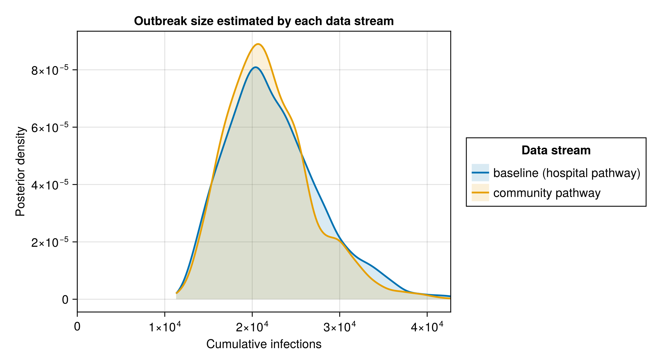
Tree-prior sensitivity
The outbreak-age estimate depends on the coalescent tree prior assumed in the BEAST X analysis. The baseline uses the more flexible Skygrid non-parametric model, which dates the common ancestor to 15 March 2026 (
Re-fit the joint under the Exponential growth tree prior
# The Exponential-growth re-fit (and its `tmrca_days` offset) is defined in the fit
# registry (`docs/fits/registry.jl`) and loaded through the cache (when enabled) in the
# setup block above.
posterior_C_exp_growth = RUN_SENSITIVITY ?
    vec(Array(chn_joint_exp_growth_clock[:C_T])) : nothing
T_skygrid = vec(Array(chn_joint[:T]))
T_exp_growth = RUN_SENSITIVITY ? vec(Array(chn_joint_exp_growth_clock[:T])) : nothing;
A slightly earlier common ancestor (Exponential growth) permits a marginally older outbreak, though the difference is small because the evolutionary rates are nearly identical.
Tree-prior infection-count table
clock_sensitivity_C_table = RUN_SENSITIVITY ?
    streams_table(
        "Skygrid (baseline)" => posterior_C_joint,
        "Exponential growth" => posterior_C_exp_growth
    ) :
Markdown.md"_Tree-prior sensitivity analysis not shown in this build._";| Stream | Lower 90% | Lower 60% | Lower 30% | Upper 30% | Upper 60% | Upper 90% |
|---|---|---|---|---|---|---|
| Skygrid (baseline) | 14896 | 17752 | 19852 | 23821 | 26643 | 32793 |
| Exponential growth | 15332 | 18051 | 19991 | 24118 | 26674 | 32379 |
Tree-prior infection-count density plot
clock_sensitivity_C_fig = RUN_SENSITIVITY ?
    plot_cumulative_cases(
        "Skygrid (baseline)" => posterior_C_joint,
        "Exponential growth" => posterior_C_exp_growth; scenarios = []
    ) :
    Markdown.md"_Tree-prior sensitivity analysis not shown in this build._";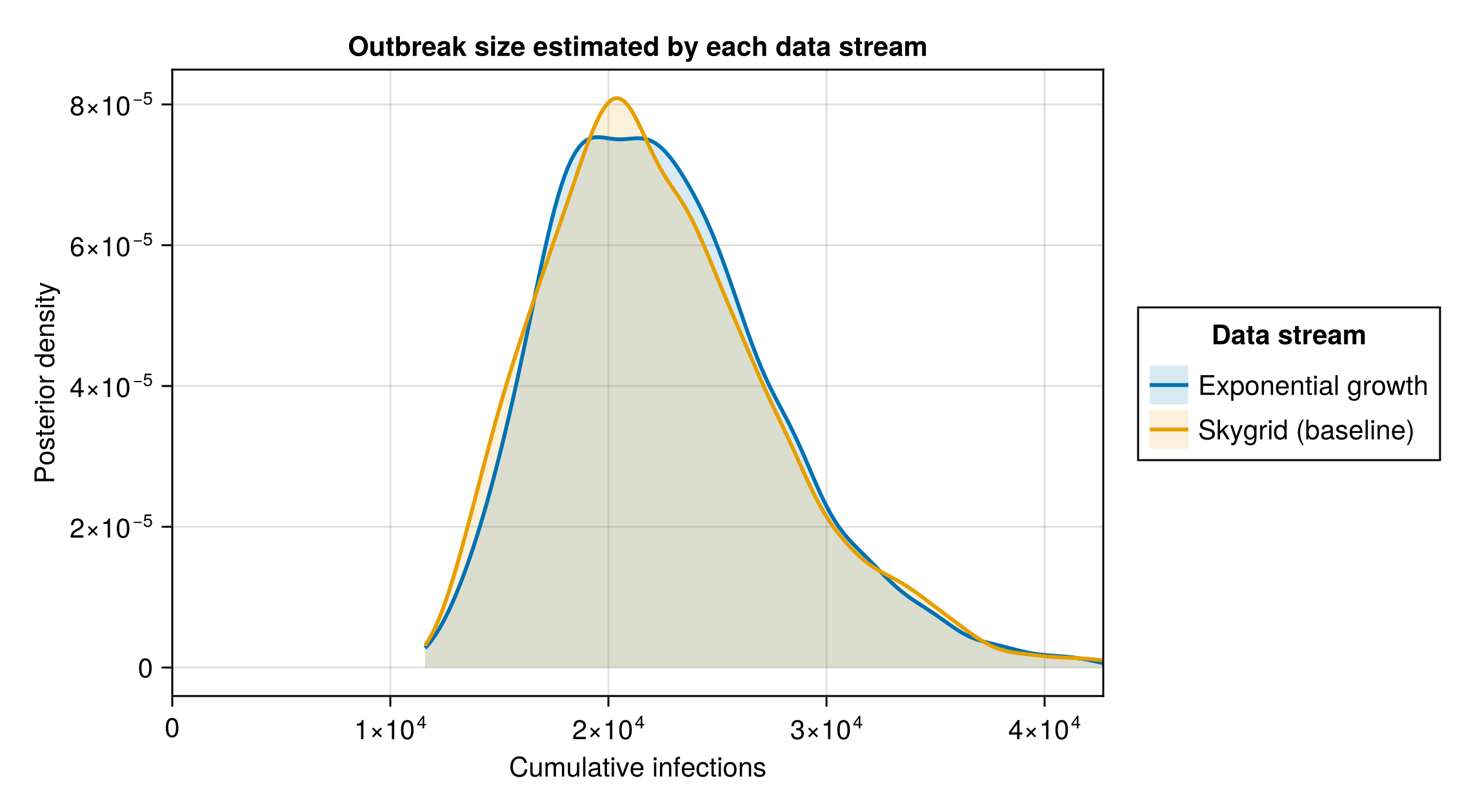
Tree-prior outbreak-age table
clock_sensitivity_T_table = RUN_SENSITIVITY ?
    streams_table(
        "Skygrid (baseline)" => T_skygrid,
        "Exponential growth" => T_exp_growth; digits = 0
    ) :
Markdown.md"_Tree-prior sensitivity analysis not shown in this build._";| Stream | Lower 90% | Lower 60% | Lower 30% | Upper 30% | Upper 60% | Upper 90% |
|---|---|---|---|---|---|---|
| Skygrid (baseline) | 206 | 211 | 214 | 221 | 225 | 234 |
| Exponential growth | 214 | 217 | 220 | 226 | 231 | 240 |
Tree-prior outbreak-age density plot
clock_sensitivity_T_fig = RUN_SENSITIVITY ?
    plot_density_overlay(
        "Skygrid (baseline)" => T_skygrid,
        "Exponential growth" => T_exp_growth;
        xlabel = "Outbreak age (days before cut-off)",
        title = "Posterior outbreak age by tree prior", lower = 0
    ) :
    Markdown.md"_Tree-prior sensitivity analysis not shown in this build._";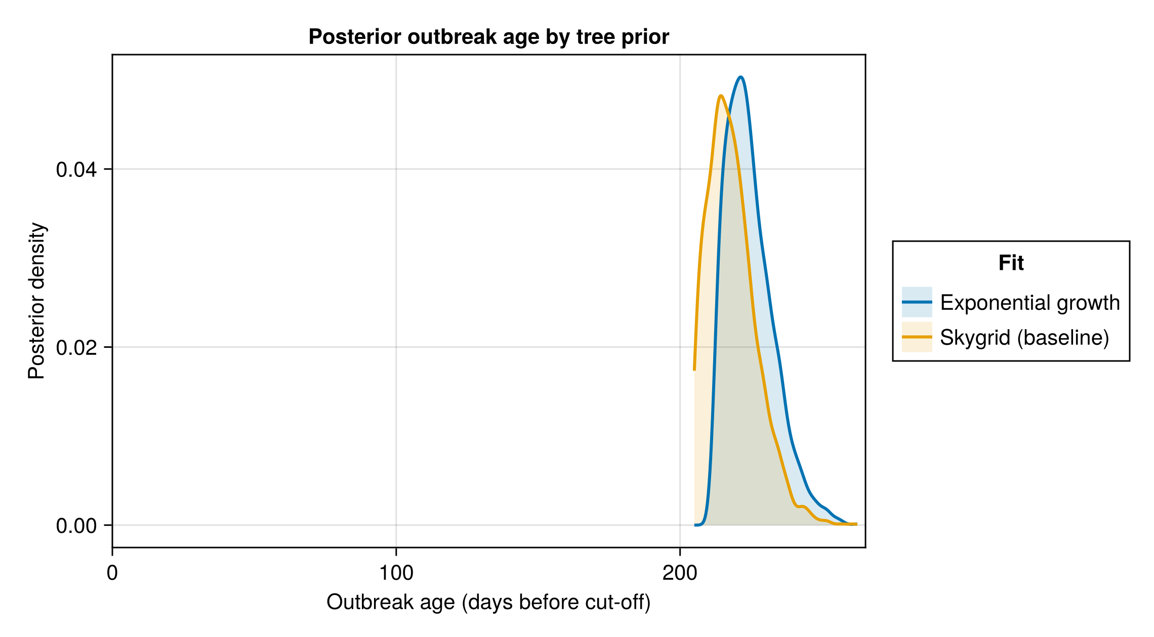
Fit diagnostics by parameter
One parameter or the whole model
Per-parameter diagnostics for every fit
# R-hat and both effective sample sizes over several thousand parameters
# are not free to compute, so each fit's per-parameter frame is built once
# here and handed to every table and figure in this section.
diagnostic_fits = [
    "joint" => chn_joint,
    "joint, no patches" => chn_no_patches,
    "exports" => chn_exports,
    "deaths (DRC)" => chn_deaths,
    "cases (DRC)" => chn_cases,
    "confirmed (DRC)" => chn_confirmed,
    "confirmed deaths (DRC)" => chn_confirmed_deaths,
    "isolation (DRC)" => chn_treatment,
    "onsets (DRC)" => chn_onsets,
    "frozen (1wk back)" => frozen_lastweek.chn,
    (
        RUN_SENSITIVITY ?
            [
                "delay sensitivity" => chn_joint_community_delay,
                "clock sensitivity (ExpGrowth)" => chn_joint_exp_growth_clock,
            ] :
            []
    )...,
]
diagnostic_frames = [
    label => parameter_diagnostics(chn)
        for (label, chn) in diagnostic_fits
]
diagnostic_frame = Dict(diagnostic_frames)
joint_diagnostics = diagnostic_frame["joint"]
diagnostic_spread = MarkdownTable(
    diagnostic_spread_table(diagnostic_frames...; labels = display_names)
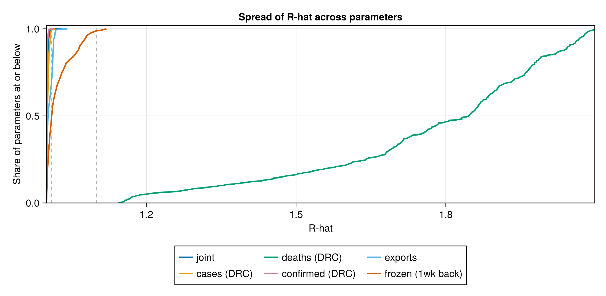
);| fit | parameters | rhat_above_1.01 | rhat_above_1.1 | percent_above_1.1 | ess_bulk_below_100 | lowest_ess_parameter |
|---|---|---|---|---|---|---|
| joint | 13341 | 40 | 0 | 0 | 3 | Rt step size |
| joint, no patches | 2306 | 0 | 0 | 0 | 0 | Rt step size |
| exports | 321 | 100 | 0 | 0 | 1 | Rt step size |
| deaths (DRC) | 560 | 560 | 560 | 100 | 472 | Rt step size |
| cases (DRC) | 564 | 6 | 0 | 0 | 0 | Rt step size |
| confirmed (DRC) | 483 | 1 | 0 | 0 | 1 | Rt step size |
| confirmed deaths (DRC) | 492 | 0 | 0 | 0 | 0 | Rt step size |
| isolation (DRC) | 378 | 36 | 0 | 0 | 1 | Rt step size |
| onsets (DRC) | 547 | 8 | 0 | 0 | 1 | Rt step size |
| frozen (1wk back) | 12879 | 6556 | 149 | 1.2 | 3501 | province_capacity_share |
| delay sensitivity | 13348 | 710 | 1 | 0 | 25 | Rt step size |
| clock sensitivity (ExpGrowth) | 13552 | 19 | 0 | 0 | 2 | σ_level |
R-hat spread figure
rhat_spread_fig = plot_rhat_spread(
    "joint" => joint_diagnostics,
    "cases (DRC)" => diagnostic_frame["cases (DRC)"],
    "deaths (DRC)" => diagnostic_frame["deaths (DRC)"],
    "confirmed (DRC)" => diagnostic_frame["confirmed (DRC)"],
    "exports" => diagnostic_frame["exports"],
    "frozen (1wk back)" => diagnostic_frame["frozen (1wk back)"]
);
Which parameters mix worst
Worst-mixing parameters of the joint fit
joint_worst_parameters = MarkdownTable(
    worst_parameters_table(
        joint_diagnostics; n = 15,
        labels = display_names
    )
);| parameter | rhat | ess_bulk | ess_tail |
|---|---|---|---|
| Rt step size | 1.032 | 60 | 60 |
| σ_level | 1.019 | 77 | 118 |
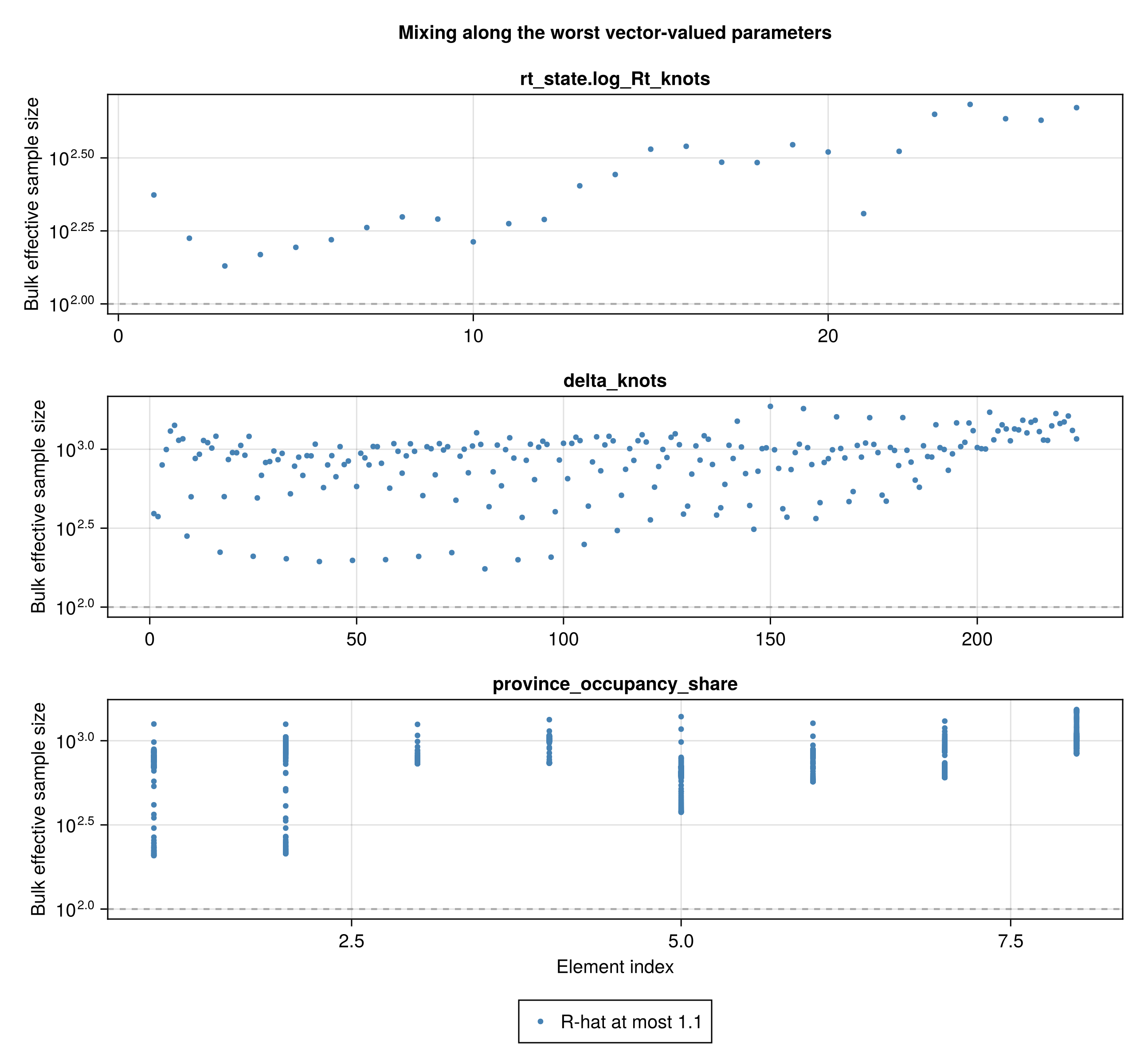
| rt_state.log_Rt_knots[3] | 1.02 | 135 | 235 |
| rt_state.log_Rt_knots[4] | 1.018 | 148 | 177 |
| rt_state.log_Rt_knots[5] | 1.019 | 156 | 240 |
| rt_state.log_Rt_knots[10] | 1.018 | 163 | 344 |
| rt_state.log_Rt_knots[6] | 1.014 | 166 | 317 |
| rt_state.log_Rt_knots[2] | 1.011 | 168 | 176 |
| delta_knots[81] | 1.018 | 175 | 374 |
| rt_state.log_Rt_knots[7] | 1.01 | 183 | 381 |
| rt_state.log_Rt_knots[11] | 1.015 | 188 | 416 |
| delta_knots[41] | 1.014 | 194 | 302 |
| rt_state.log_Rt_knots[12] | 1.014 | 195 | 385 |
| rt_state.log_Rt_knots[9] | 1.013 | 195 | 375 |
| delta_knots[49] | 1.012 | 198 | 405 |
Worst-mixing parameters, grouped
joint_worst_groups = MarkdownTable(
    family_diagnostics_table(
        joint_diagnostics; n = 12,
        labels = display_names
    )
);| parameter | elements | max_rhat | min_ess_bulk | above_1.1 |
|---|---|---|---|---|
| Rt step size | 1 | 1.032 | 60 | 0 |
| σ_level | 1 | 1.019 | 77 | 0 |
| rt_state.log_Rt_knots | 27 | 1.02 | 135 | 0 |
| delta_knots | 224 | 1.019 | 175 | 0 |
| province_occupancy_share | 1640 | 1.009 | 208 | 0 |
| u_level | 7 | 1.018 | 229 | 0 |
| σ_dest | 1 | 1.01 | 273 | 0 |
| importation_epsilon_patch | 8 | 1.006 | 282 | 0 |
| infections_patch | 1685 | 1.005 | 296 | 0 |
| susceptible_fraction_patch | 1685 | 1.006 | 300 | 0 |
| importation_patch | 1639 | 1.009 | 302 | 0 |
| importation_destination_effect | 8 | 1.008 | 329 | 0 |
Mixing over time-varying parameters
joint_index_fig = plot_parameter_index_diagnostics(
    joint_diagnostics;
    n_groups = 3, labels = display_names
);
Where the divergent transitions sit
Sampler behaviour by chain
joint_chain_table = MarkdownTable(sampler_by_chain_table(chn_joint));| chain | draws | divergences | percent_divergent | step_size | deepest_tree | percent_at_max_depth | mean_acceptance | ebfmi |
|---|---|---|---|---|---|---|---|---|
| 1 | 1000 | 1 | 0.1 | 0.00364 | 10 | 99.9 | 0.889 | 0.562 |
| 2 | 1000 | 0 | 0 | 0.00282 | 10 | 100 | 0.946 | 0.82 |
Divergence location table
joint_divergence_table = MarkdownTable(
    divergence_location_table(chn_joint; n = 12, labels = display_names)
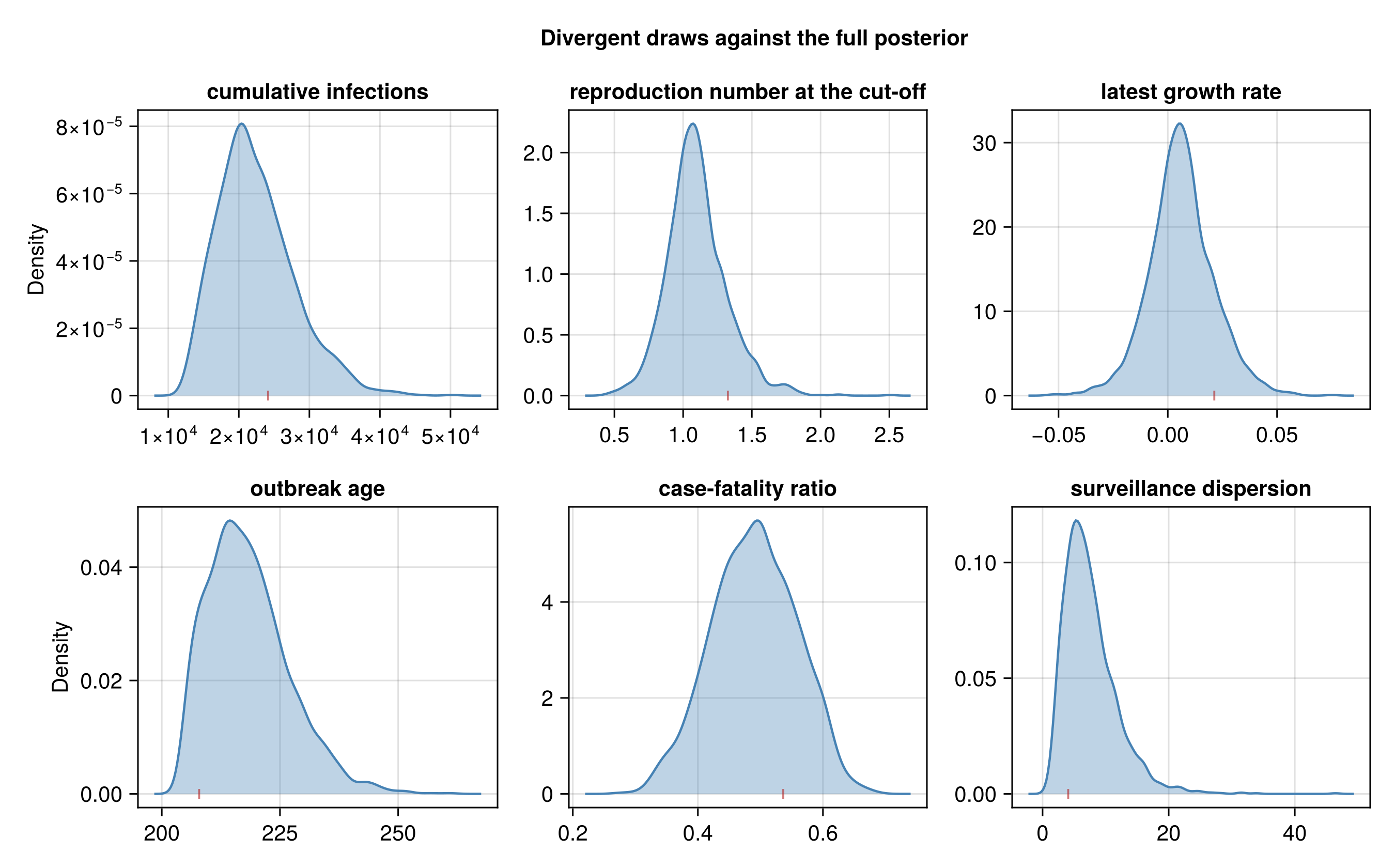
);| parameter | all_draws | divergent_draws | separation |
|---|---|---|---|
| confirmed_state.intensity_state.κ | 1.1–1.52 | 1.61–1.61 | 2.8 |
| cases_state.pos_state.τ_test | 0.718–0.971 | 0.678–0.678 | -2.64 |
| treatment_state.occupancy_break | -205.0–-102.0 | -224.0–-224.0 | -2.4 |
| treatment_state.abscond_frac | 0.0089–0.0117 | 0.00847–0.00847 | -2.08 |
| background_total | 34200.0–39800.0 | 34100.0–34100.0 | -1.93 |
| treatment_state.adm_state.p_iso | 0.293–0.351 | 0.351–0.351 | 1.88 |
| treatment_state.expected_bed_demand | 1110.0–1260.0 | 1260.0–1260.0 | 1.8 |
| treatment_state.recovery_los_state.delay_sd | 2.19–14.4 | 1.03–1.03 | -1.75 |
| confirmed_deaths_state.q_death | 0.29–0.768 | 0.726–0.726 | 1.71 |
| confirmed_deaths_state.p_death_conf | 0.29–0.717 | 0.683–0.683 | 1.68 |
| ε_bar | 0.00254–0.0265 | 0.0239–0.0239 | 1.64 |
| bg_pool.σ_bg | 0.194–0.347 | 0.334–0.334 | 1.56 |
Divergent draws against the posterior
joint_divergence_fig = plot_divergence_locations(
    chn_joint,
    [:C_T, :R_T, :r, :T, :CFR, :k];
    labels = Dict(
        :C_T => "cumulative infections",
        :R_T => "reproduction number at the cut-off",
        :r => "latest growth rate", :T => "outbreak age",
        :CFR => "case-fatality ratio",
        :k => "surveillance dispersion"
    )
);
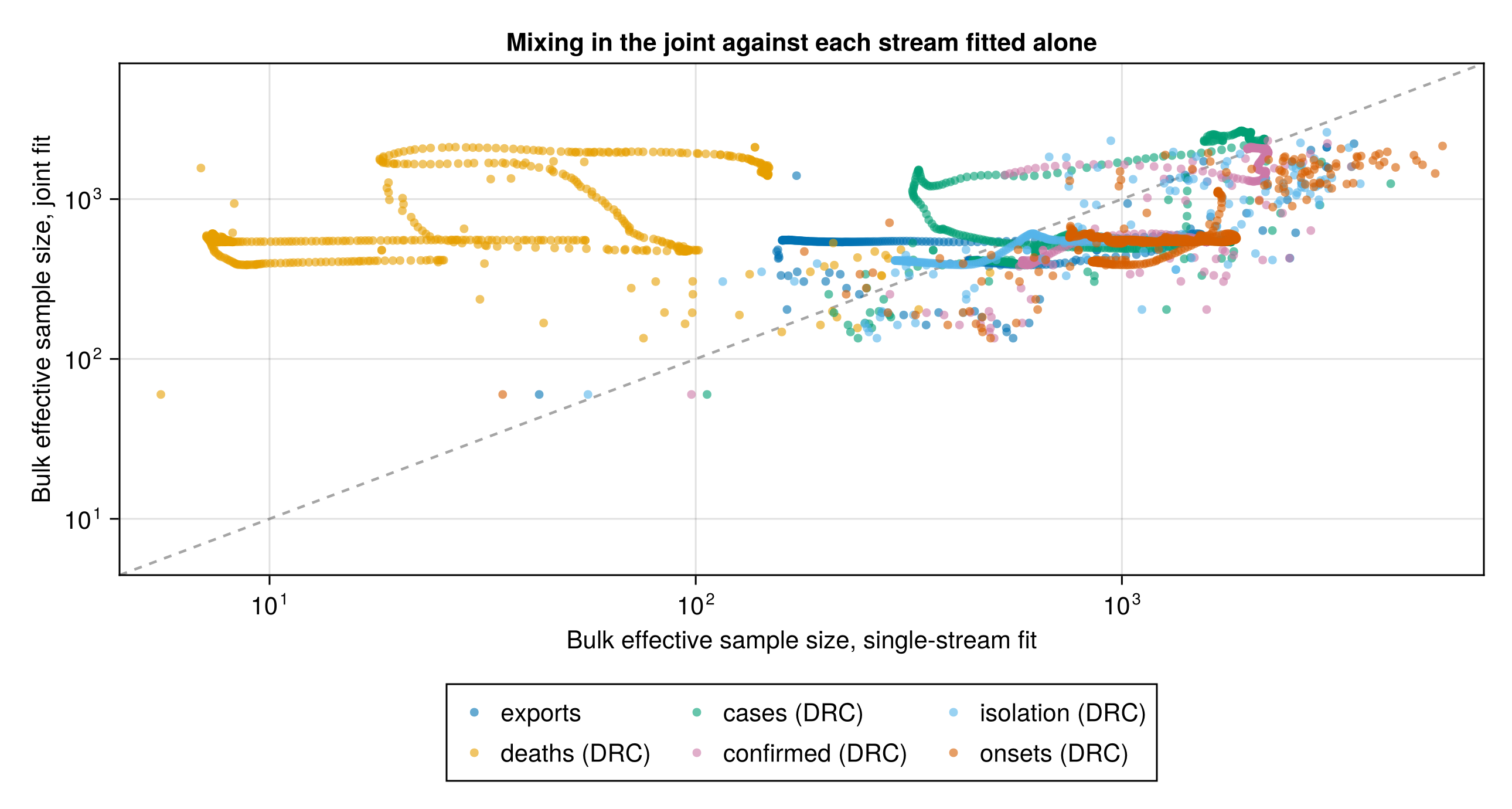
The joint fit against the single-stream fits
Joint against single-stream contrast
stream_contrast = diagnostic_contrast(
    "joint" => joint_diagnostics,
    "exports" => diagnostic_frame["exports"],
    "deaths (DRC)" => diagnostic_frame["deaths (DRC)"],
    "cases (DRC)" => diagnostic_frame["cases (DRC)"],
    "confirmed (DRC)" => diagnostic_frame["confirmed (DRC)"],
    "isolation (DRC)" => diagnostic_frame["isolation (DRC)"],
    "onsets (DRC)" => diagnostic_frame["onsets (DRC)"]
)
stream_contrast_table = MarkdownTable(
    diagnostic_contrast_table(
        stream_contrast; n = 15,
        labels = display_names
    )
);| fit | parameter | ess_bulk | ess_bulk_reference | ess_ratio |
|---|---|---|---|---|
| confirmed (DRC) | rt_state.log_Rt_knots[21] | 1581 | 204 | 0.13 |
| cases (DRC) | rt_state.log_Rt_knots[21] | 1272 | 204 | 0.16 |
| exports | asc_state.p_drc | 2479 | 427 | 0.17 |
| confirmed (DRC) | asc_state.p_drc | 2472 | 427 | 0.17 |
| confirmed (DRC) | rt_state.log_Rt_knots[18] | 1731 | 305 | 0.18 |
| isolation (DRC) | rt_state.log_Rt_knots[21] | 1114 | 204 | 0.18 |
| isolation (DRC) | confirmed_state.s_test | 2256 | 416 | 0.18 |
| confirmed (DRC) | rt_state.log_Rt_knots[20] | 1757 | 331 | 0.19 |
| confirmed (DRC) | confirmed_state.s_test | 2140 | 416 | 0.19 |
| confirmed (DRC) | rt_state.log_Rt_knots[22] | 1643 | 333 | 0.2 |
| cases (DRC) | rt_state.log_Rt_knots[22] | 1540 | 333 | 0.22 |
| isolation (DRC) | treatment_state.isolation_bvd_admission | 1774 | 390 | 0.22 |
| isolation (DRC) | treatment_state.adm_state.p_iso | 2058 | 456 | 0.22 |
| confirmed (DRC) | rt_state.log_Rt_knots[17] | 1375 | 306 | 0.22 |
| confirmed (DRC) | rt_state.log_Rt_knots[19] | 1561 | 351 | 0.22 |
Joint against single-stream figure
stream_contrast_fig = plot_diagnostic_contrast(
    stream_contrast;
    xlabel = "Bulk effective sample size, single-stream fit",
    ylabel = "Bulk effective sample size, joint fit",
    title = "Mixing in the joint against each stream fitted alone"
);
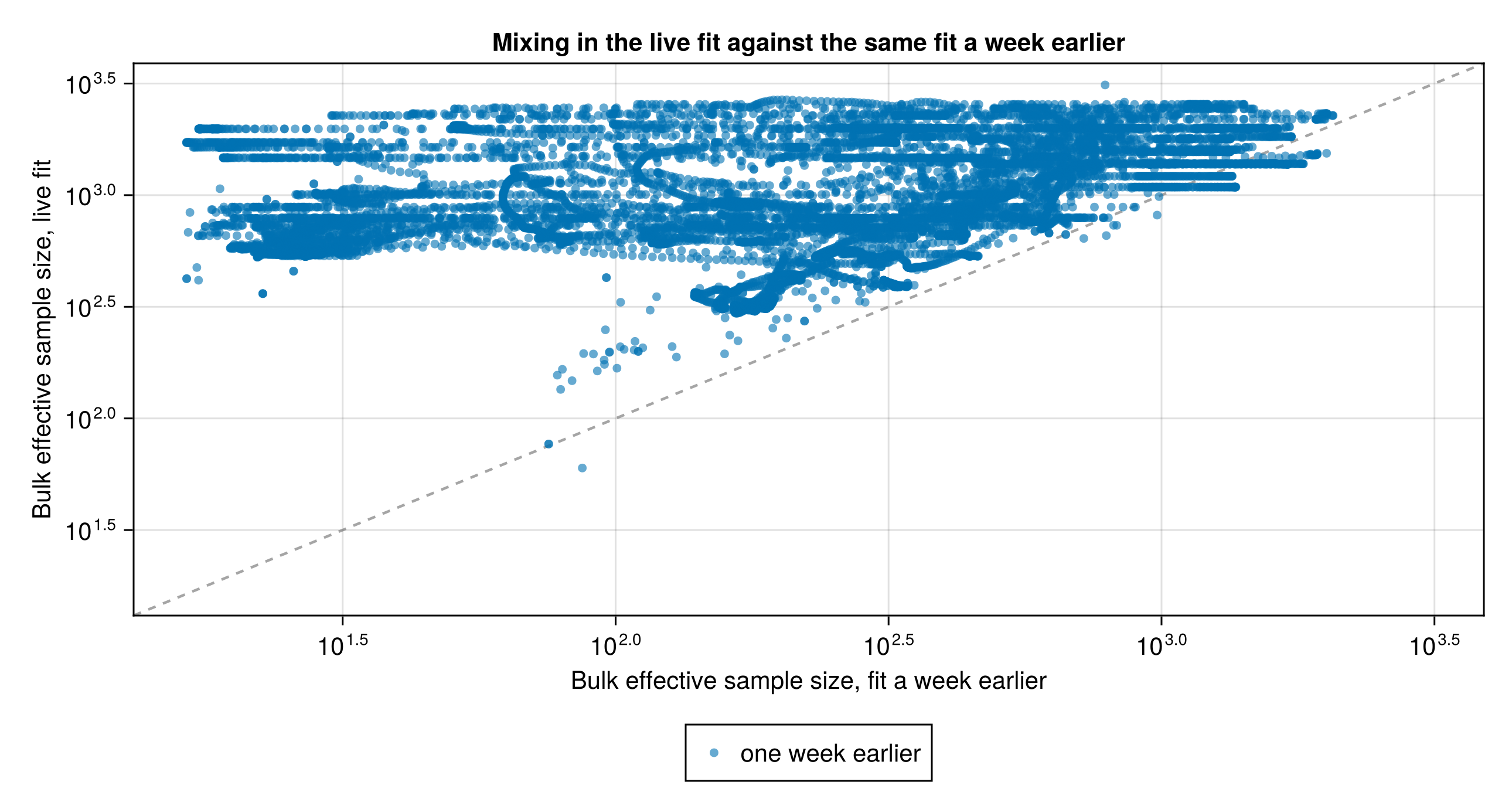
The joint fit against the same fit a week earlier
Live against frozen contrast
frozen_contrast = diagnostic_contrast(
    "joint" => joint_diagnostics,
    "one week earlier" => diagnostic_frame["frozen (1wk back)"]
)
frozen_contrast_table = MarkdownTable(
    diagnostic_contrast_table(
        frozen_contrast; n = 15,
        labels = display_names
    )
);| fit | parameter | ess_bulk | ess_bulk_reference | ess_ratio |
|---|---|---|---|---|
| one week earlier | Rt step size | 87 | 60 | 0.69 |
| one week earlier | province_shares[4] | 1819 | 1382 | 0.76 |
| one week earlier | province_shares[4] | 1819 | 1382 | 0.76 |
| one week earlier | province_shares[4] | 1811 | 1382 | 0.76 |
| one week earlier | province_shares[4] | 1810 | 1382 | 0.76 |
| one week earlier | province_shares[4] | 1808 | 1382 | 0.76 |
| one week earlier | province_shares[4] | 1801 | 1382 | 0.77 |
| one week earlier | expected_onset_reported_T | 2007 | 1540 | 0.77 |
| one week earlier | province_shares[4] | 1798 | 1382 | 0.77 |
| one week earlier | province_shares[4] | 1795 | 1382 | 0.77 |
| one week earlier | province_shares[4] | 1781 | 1382 | 0.78 |
| one week earlier | province_shares[4] | 1769 | 1382 | 0.78 |
| one week earlier | province_shares[4] | 1762 | 1382 | 0.78 |
| one week earlier | cumulative_confirmed_deaths[242] | 1926 | 1519 | 0.79 |
| one week earlier | cumulative_confirmed_deaths[241] | 1922 | 1517 | 0.79 |
Live against frozen figure
frozen_contrast_fig = plot_diagnostic_contrast(
    frozen_contrast;
    xlabel = "Bulk effective sample size, fit a week earlier",
    ylabel = "Bulk effective sample size, live fit",
    title = "Mixing in the live fit against the same fit a week earlier"
);
Parameter recovery
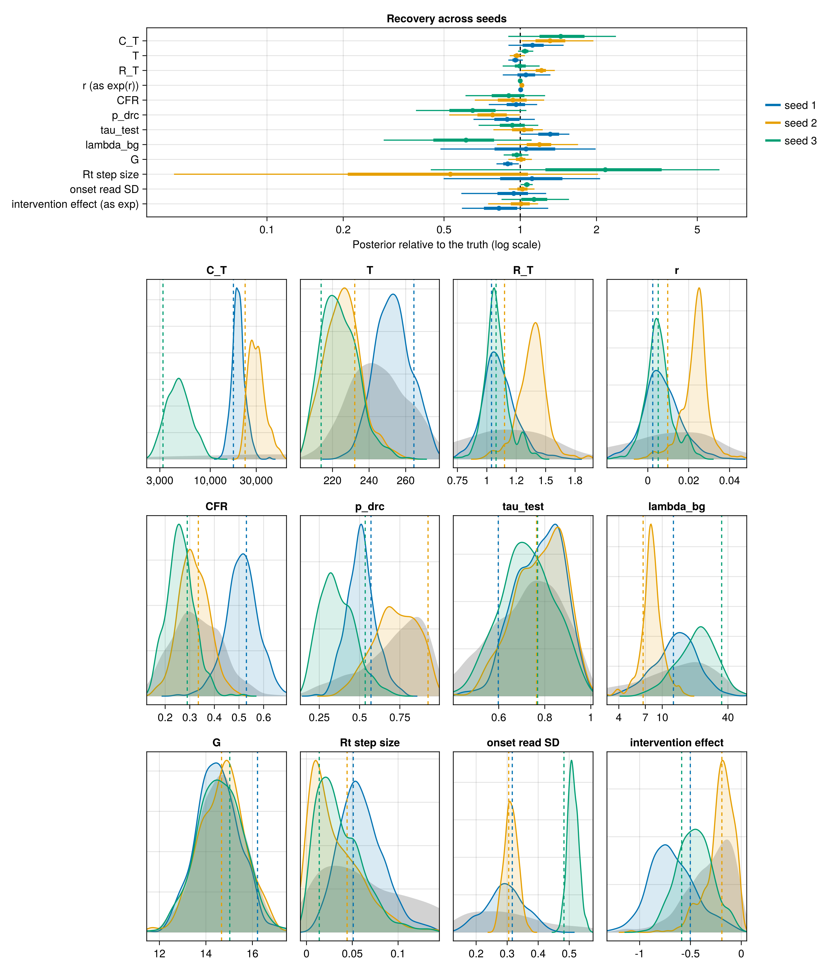
Whether the model recovers known values when fitted to data it simulated itself. Each seed is one prior draw of the model run past the cut-off, kept when its outbreak size is within a factor of five of the one observed, and fitted with the headline joint's sampler settings.
Recovery figure
recovery = recovery_results()
recovery_national_quantities = [
    "C_T", "T", "R_T", "r", "CFR", "p_drc", "tau_test", "lambda_bg",
    "growth_state.G", "rt_state.sigma_rw", "onset_report_state.τ",
    "rt_state.intervention_effect",
]
recovery_labels = Dict(
    "growth_state.G" => "G", "rt_state.sigma_rw" => "Rt step size",
    "onset_report_state.τ" => "onset read SD",
    "rt_state.intervention_effect" => "intervention effect",
)
recovery_fig = isempty(recovery.params) ? nothing : plot_recovery(
        recovery.params, recovery.draws, recovery.prior;
        quantities = recovery_national_quantities,
        labels = merge(
            recovery_labels,
            Dict(
                "r" => "r (as exp(r))",
                "rt_state.intervention_effect" => "intervention effect (as exp)",
            )
        ),
        panel_labels = merge(recovery_labels, Dict("r" => "r")),
        log_x = ["C_T", "lambda_bg"],
        difference = ["r", "rt_state.intervention_effect"]
    );
Summary table across seeds
recovery_summary_national = isempty(recovery.params) ? DataFrame() :
    recovery_summary_table(recovery.params; province = false);

recovery_summary_national_display = isempty(recovery_summary_national) ?
    Markdown.parse("No parameter-recovery run is available for this build.") :
MarkdownTable(recovery_summary_national);| Quantity | Truth, lowest | Truth, highest | Relative error, median | Relative error, range | z, median | Truth in 90% | Outside 99% |
|---|---|---|---|---|---|---|---|
| CFR | 0.29 | 0.53 | -0.06 | -0.1 to -0.04 | -0.32 | 3/3 | 0 |
| C_T | 3230 | 23000 | 0.31 | 0.12 to 0.44 | 1.13 | 2/3 | 0 |
| R_T | 1.04 | 1.15 | 0.05 | -0.0 to 0.21 | 0.47 | 2/3 | 0 |
| T | 214 | 264 | -0.03 | -0.04 to 0.04 | -0.7 | 3/3 | 0 |
| growth_state.G | 14.7 | 16.2 | -0.03 | -0.11 to 0.01 | -0.46 | 2/3 | 0 |
| lambda_bg | 6.68 | 35 | 0.05 | -0.39 to 0.19 | 0.25 | 3/3 | 0 |
| onset_report_state.τ | 0.305 | 0.483 | 0.02 | -0.06 to 0.06 | 0.29 | 2/3 | 0 |
| p_drc | 0.535 | 0.925 | -0.22 | -0.35 to -0.11 | -1.56 | 2/3 | 0 |
| r | 0.00242 | 0.00974 | 1.48 | -0.03 to 1.63 | 0.47 | 2/3 | 0 |
| rt_state.intervention_effect | -0.586 | -0.191 | 0.04 | -0.39 to 0.21 | -0.11 | 3/3 | 0 |
| rt_state.sigma_rw | 0.0139 | 0.0511 | 0.11 | -0.47 to 1.17 | 0.37 | 3/3 | 0 |
| tau_test | 0.598 | 0.769 | 0.03 | -0.07 to 0.31 | 0.16 | 2/3 | 0 |
Each seed's fit and recovered values
recovery_seeds = isempty(recovery.params) ? DataFrame() :
    recovery_seed_verdicts(recovery.params);
recovery_national = isempty(recovery.params) ? DataFrame() :
    recovery.params[
        .!occursin.("[", recovery.params.quantity), [
            :seed, :quantity, :truth, :median, :lower_90, :upper_90, :covered_90,
        ],
    ];

recovery_seeds_display = isempty(recovery_seeds) ?
    Markdown.parse("No parameter-recovery run is available for this build.") :
    MarkdownTable(recovery_seeds);
recovery_national_display = isempty(recovery_national) ? Markdown.parse("") :
MarkdownTable(recovery_national);| seed | status | coverage_90 | outside | fit_minutes | max_rhat | min_ess_bulk | divergences |
|---|---|---|---|---|---|---|---|
| 1 | pass | 0.904 | 244.1 | 1.018 | 81.438 | 39 | |
| 2 | unconverged | 0.846 | 245.7 | 1.185 | 13.769 | 19 | |
| 3 | unconverged | 0.904 | 134.9 | 1.086 | 20.43 | 11 |
| seed | quantity | truth | median | lower_90 | upper_90 | covered_90 |
|---|---|---|---|---|---|---|
| 1 | CFR | 0.53 | 0.511 | 0.398 | 0.618 | true |
| 1 | C_T | 17390.379 | 19439.212 | 15622.521 | 25788.455 | true |
| 1 | R_T | 1.04 | 1.095 | 0.887 | 1.368 | true |
| 1 | T | 264.496 | 253.107 | 237.292 | 270.807 | true |
| 1 | growth_state.G | 16.22 | 14.475 | 13.067 | 16.002 | false |
| 1 | lambda_bg | 12.659 | 13.346 | 6.128 | 25.119 | true |
| 1 | onset_report_state.τ | 0.316 | 0.298 | 0.185 | 0.4 | true |
| 1 | p_drc | 0.571 | 0.507 | 0.373 | 0.652 | true |
| 1 | r | 0.00242 | 0.00638 | -0.00783 | 0.0234 | true |
| 1 | rt_state.intervention_effect | -0.502 | -0.695 | -1.032 | -0.247 | true |
| 1 | rt_state.sigma_rw | 0.0511 | 0.0568 | 0.0254 | 0.106 | true |
| 1 | tau_test | 0.598 | 0.785 | 0.601 | 0.935 | false |
| 2 | CFR | 0.335 | 0.313 | 0.222 | 0.416 | true |
| 2 | C_T | 23004.974 | 30178.71 | 23279.601 | 44732.351 | false |
| 2 | R_T | 1.15 | 1.396 | 1.161 | 1.575 | false |
| 2 | T | 232.161 | 225.017 | 210.902 | 242.114 | true |
| 2 | growth_state.G | 14.674 | 14.787 | 13.16 | 16.307 | true |
| 2 | lambda_bg | 6.681 | 7.959 | 5.405 | 11.299 | true |
| 2 | onset_report_state.τ | 0.305 | 0.311 | 0.275 | 0.347 | true |
| 2 | p_drc | 0.925 | 0.719 | 0.485 | 0.921 | false |
| 2 | r | 0.00974 | 0.0241 | 0.0105 | 0.0321 | false |
| 2 | rt_state.intervention_effect | -0.191 | -0.184 | -0.483 | -0.0286 | true |
| 2 | rt_state.sigma_rw | 0.0443 | 0.0235 | 0.0019 | 0.0898 | true |
| 2 | tau_test | 0.764 | 0.791 | 0.599 | 0.938 | true |
| 3 | CFR | 0.29 | 0.261 | 0.176 | 0.363 | true |
| 3 | C_T | 3234.286 | 4673.472 | 2901.052 | 7719.564 | true |
| 3 | R_T | 1.079 | 1.074 | 0.919 | 1.286 | true |
| 3 | T | 213.788 | 223.161 | 209.544 | 240.672 | true |
| 3 | growth_state.G | 15.027 | 14.554 | 12.922 | 16.197 | true |
| 3 | lambda_bg | 35.032 | 21.398 | 10.123 | 38.84 | true |
| 3 | onset_report_state.τ | 0.483 | 0.513 | 0.485 | 0.541 | false |
| 3 | p_drc | 0.535 | 0.347 | 0.207 | 0.566 | true |
| 3 | r | 0.00509 | 0.00496 | -0.00593 | 0.018 | true |
| 3 | rt_state.intervention_effect | -0.586 | -0.461 | -0.757 | -0.143 | true |
| 3 | rt_state.sigma_rw | 0.0139 | 0.0302 | 0.00617 | 0.0852 | true |
| 3 | tau_test | 0.769 | 0.715 | 0.526 | 0.906 | true |
Forecast scores from the recovery fits
recovery_forecasts = isempty(recovery.forecasts) ? DataFrame() :
    recovery.forecasts[
        :, [
            :seed, :horizon, :quantity, :truth, :baseline, :crps, :baseline_crps,
            :relative_crps, :covered_90,
        ],
    ];

recovery_forecasts_display = isempty(recovery_forecasts) ?
    Markdown.parse("No recovery forecast is available for this build.") :
MarkdownTable(recovery_forecasts);| seed | horizon | quantity | truth | baseline | crps | baseline_crps | relative_crps | covered_90 |
|---|---|---|---|---|---|---|---|---|
| 1 | 7 | confirmed_deaths_new | 211 | 245 | 19.336 | 34 | 0.569 | true |
| 1 | 7 | confirmed_new | 206 | 2618 | 28.575 | 2412 | 0.0118 | true |
| 1 | 14 | confirmed_deaths_new | 474 | 486 | 22.126 | 12 | 1.844 | true |
| 1 | 14 | confirmed_new | 459 | 4993 | 36.916 | 4534 | 0.00814 | true |
| 2 | 7 | confirmed_deaths_new | 777 | 778 | 106.777 | 1 | 106.777 | true |
| 2 | 7 | confirmed_new | 2846 | 3123 | 278.733 | 277 | 1.006 | true |
| 2 | 14 | confirmed_deaths_new | 1478 | 1703 | 425.542 | 225 | 1.891 | false |
| 2 | 14 | confirmed_new | 4351 | 5826 | 1111.598 | 1475 | 0.754 | true |
| 3 | 7 | confirmed_deaths_new | 47 | 33 | 6.431 | 14 | 0.459 | true |
| 3 | 7 | confirmed_new | 29 | 1959 | 25.446 | 1930 | 0.0132 | false |
| 3 | 14 | confirmed_deaths_new | 75 | 69 | 3.815 | 6 | 0.636 | true |
| 3 | 14 | confirmed_new | 122 | 3602 | 8.987 | 3480 | 0.00258 | true |
Saving in-sample outputs
The per-stream infection-count table is written to the shared output directory.
Write in-sample outputs
output_dir = get(
    ENV, "BVD_OUTPUT_DIR",
    joinpath(pkgdir(BVDOutbreakSize), "output")
)
mkpath(output_dir)
CSV.write(
    joinpath(output_dir, "cumulative_cases_by_stream.csv"),
    streams_C_table
)"/home/runner/work/BVDOutbreakSize/BVDOutbreakSize/output/cumulative_cases_by_stream.csv"Write the summary bullets
dashboard_dir = joinpath(
    pkgdir(BVDOutbreakSize), "docs", "src", "summary_assets"
)
mkpath(dashboard_dir)

# The bullets under the summary heading at the top of the page. They read
# tables built further down, so they are written here and read back when
# the site is assembled.
evaluation_insample_national_summary = let
    fmt(x) = ismissing(x) || !isfinite(x) ? "n/a" :
        string(round(x; digits = 2))
    cal = filter(r -> isfinite(r["90% coverage"]), stream_calibration_table)
    n_cov = count(>=(0.8), cal[!, "90% coverage"])
    calibrated(r) = string(
        r["Stream"], " (bias ", fmt(r["Bias"]), ", 90% coverage ",
        fmt(r["90% coverage"]), ")"
    )
    worst = first(
        sort(cal, "Bias"; by = abs, rev = true), min(3, size(cal, 1))
    )
    pred(x, observed) = string(
        "observed ", observed, " against a predictive median of ",
        round(Int, quantile(x, 0.5)), " (90% interval ",
        round(Int, quantile(x, 0.05)), "–",
        round(Int, quantile(x, 0.95)), ")"
    )
    overall = [
        string(
            "- **Streams:** ", n_cov, " of ", size(cal, 1),
            " fitted streams have 90% coverage of at least 0.8."
        ),
        string(
            "- **Least well reproduced:** ",
            join(calibrated.(eachrow(worst)), "; "), "."
        ),
        string(
            "- **Exports:** Uganda exports ",
            pred(pp_exports, obs.exported_cases), ", and export deaths ",
            pred(pp_exports_deaths, obs.exports_deaths), "."
        ),
    ]
    # Per stream, split the same way as the posterior predictive checks.
    reporting = Set(p.title for p in reporting_panels)
    function block(lead, keep)
        rows = filter(r -> keep(r["Stream"] in reporting), cal)
        size(rows, 1) == 0 && return nothing
        return join(
            vcat(
                [string("**", lead, "**"), ""],
                [
                    string(
                        "- ", r["Stream"], ": bias ", fmt(r["Bias"]),
                        ", 90% coverage ", fmt(r["90% coverage"]), " over ",
                        r["Vintages"], " vintages."
                    )
                        for r in eachrow(rows)
                ]
            ), "\n"
        )
    end
    blocks = filter(
        !isnothing,
        [
            block("Streams still reporting", identity),
            block("Streams no longer reporting", !),
        ]
    )
    join(vcat([join(overall, "\n")], blocks), "\n\n")
end
write(
    joinpath(dashboard_dir, "evaluation_insample_national.md"),
    evaluation_insample_national_summary
);