Province forecasts

This page gives the one-week-ahead forecast for each province from the joint model, as defined in the province forecast Methods section. The national forecast is on the forecasts page. How these forecasts have scored against what each province went on to report is in the forecast by province evaluation. How well the model reproduces each province's share is on the in-sample checks page.

Load packages, data and fitted chains

julia

# Shared setup: packages, observations and the fit registry. See
# `docs/pages/_setup.jl`.
using BVDOutbreakSize
include(joinpath(pkgdir(BVDOutbreakSize), "docs", "pages", "_setup.jl"))

validation_forecast_from (generic function with 1 method)

julia

# The fits this page reads, loaded from the cache here.
chn_joint = load_fit("joint");

Summary

The table gives each province's forecast for the week to as a 90% predictive interval, and the bullets compare the provinces draw by draw.

Project each province a week ahead

julia

# Read from the same draws as the national forecast page, so the provinces
# add up to the national forecast shown there.
province_draws = fit_forecast("joint");
province_projection = forecast_provinces(
    province_draws; horizon = 7, n_patches = N_PATCHES
);
province_forecast = province_forecast_table(
    province_draws, province_projection;
    n_patches = N_PATCHES
);
province_forecast_fig = plot_province_forecast(
    province_draws, province_projection;
    n_patches = N_PATCHES
);
province_week_end = obs.cutoff + Day(7);
province_forecast_md = province_forecast_headline(
    province_projection; n_patches = N_PATCHES
);

Province	New confirmed cases	New confirmed deaths	Patients in isolation	Isolation beds	New infections	R at T+7	P(R > 1)
Ituri	207–534	72–201	394–946	570–1893	282–1273	0.69–1.6	58%
Nord-Kivu	135–395	60–175	220–636	163–541	219–1093	0.7–1.66	63%
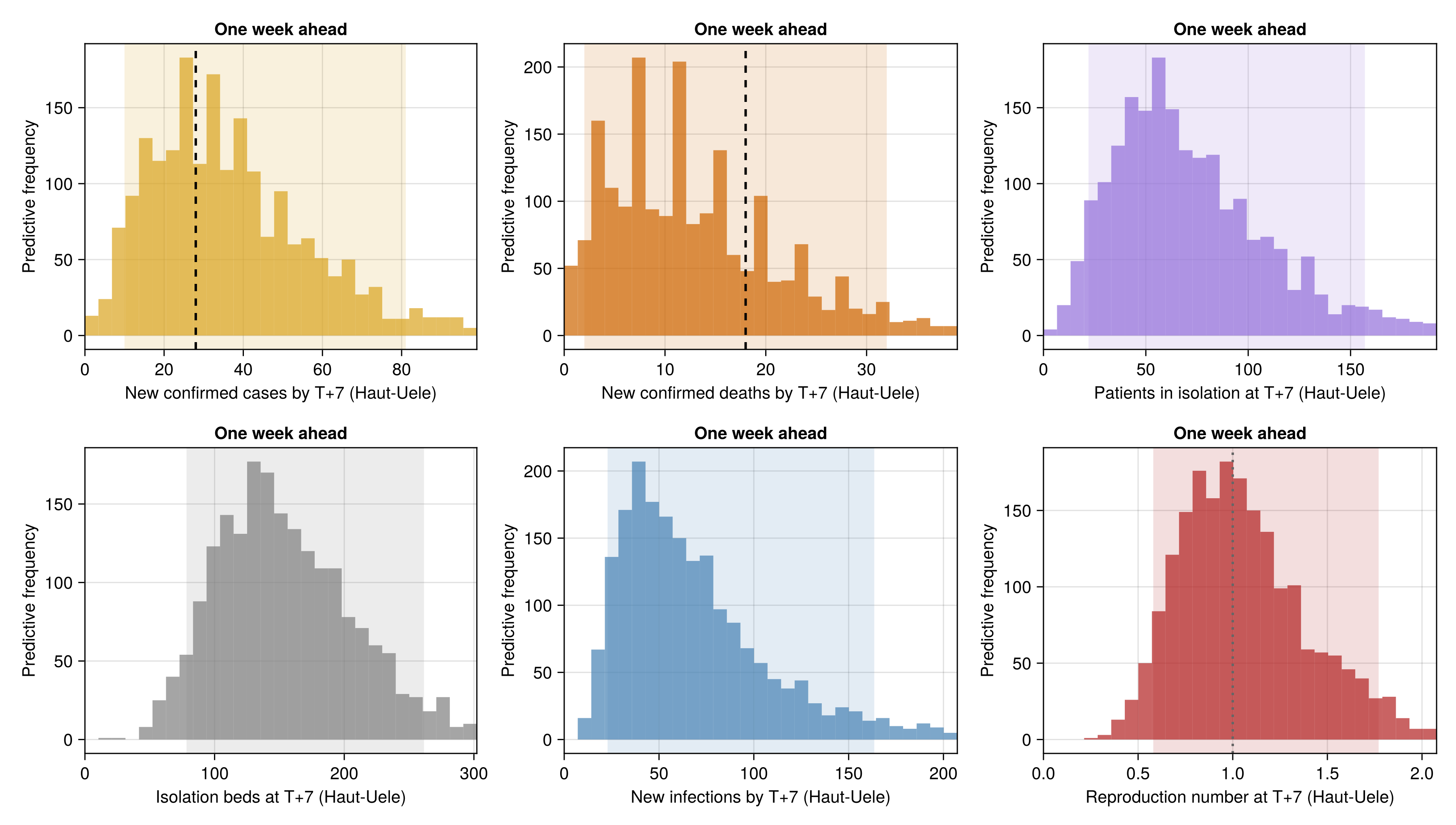
Haut-Uele	10–81	2–32	22–157	78–261	23–164	0.58–1.77	52%
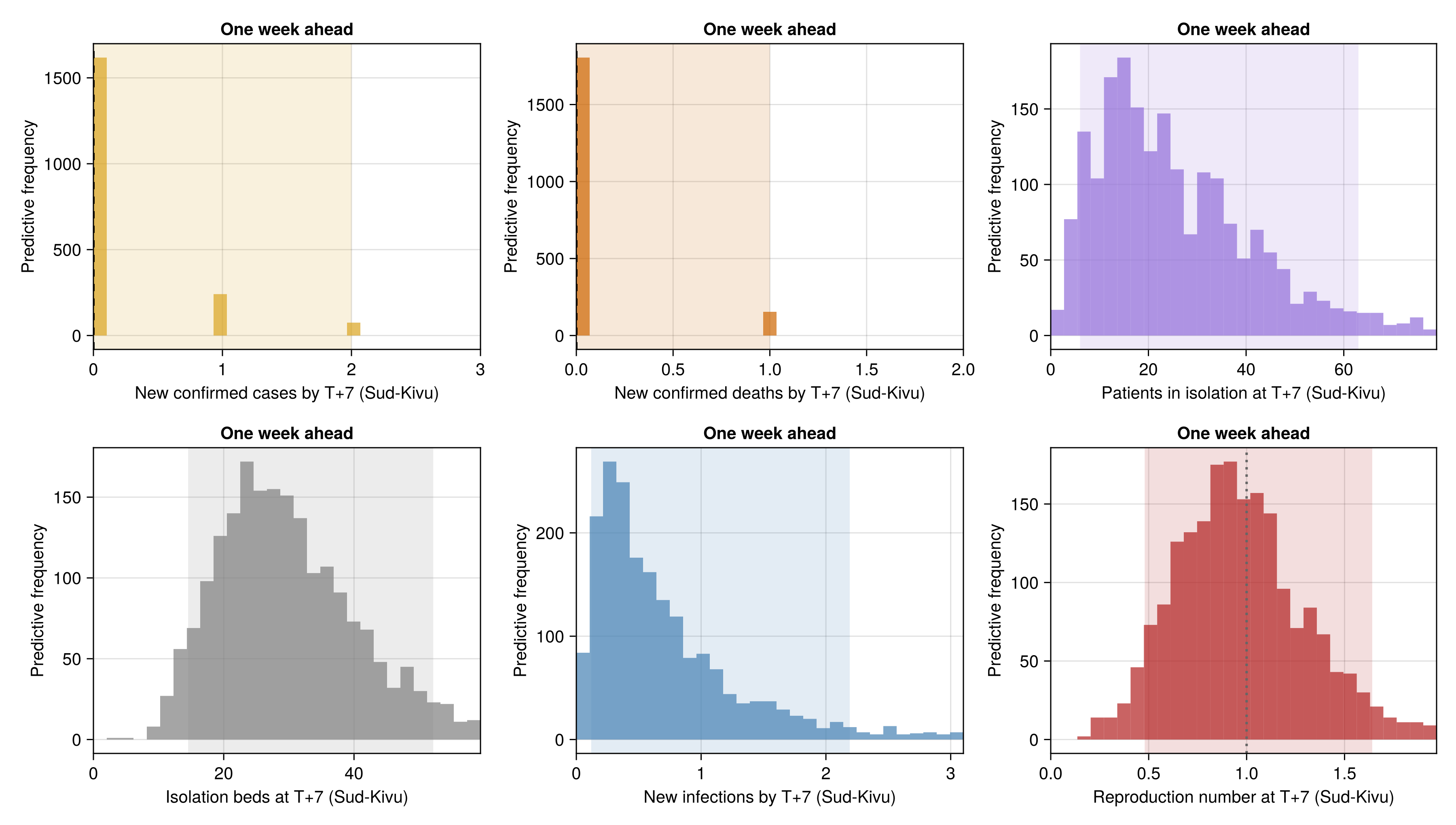
Sud-Kivu	0–2	0–1	6–63	15–52	0–2	0.48–1.64	44%
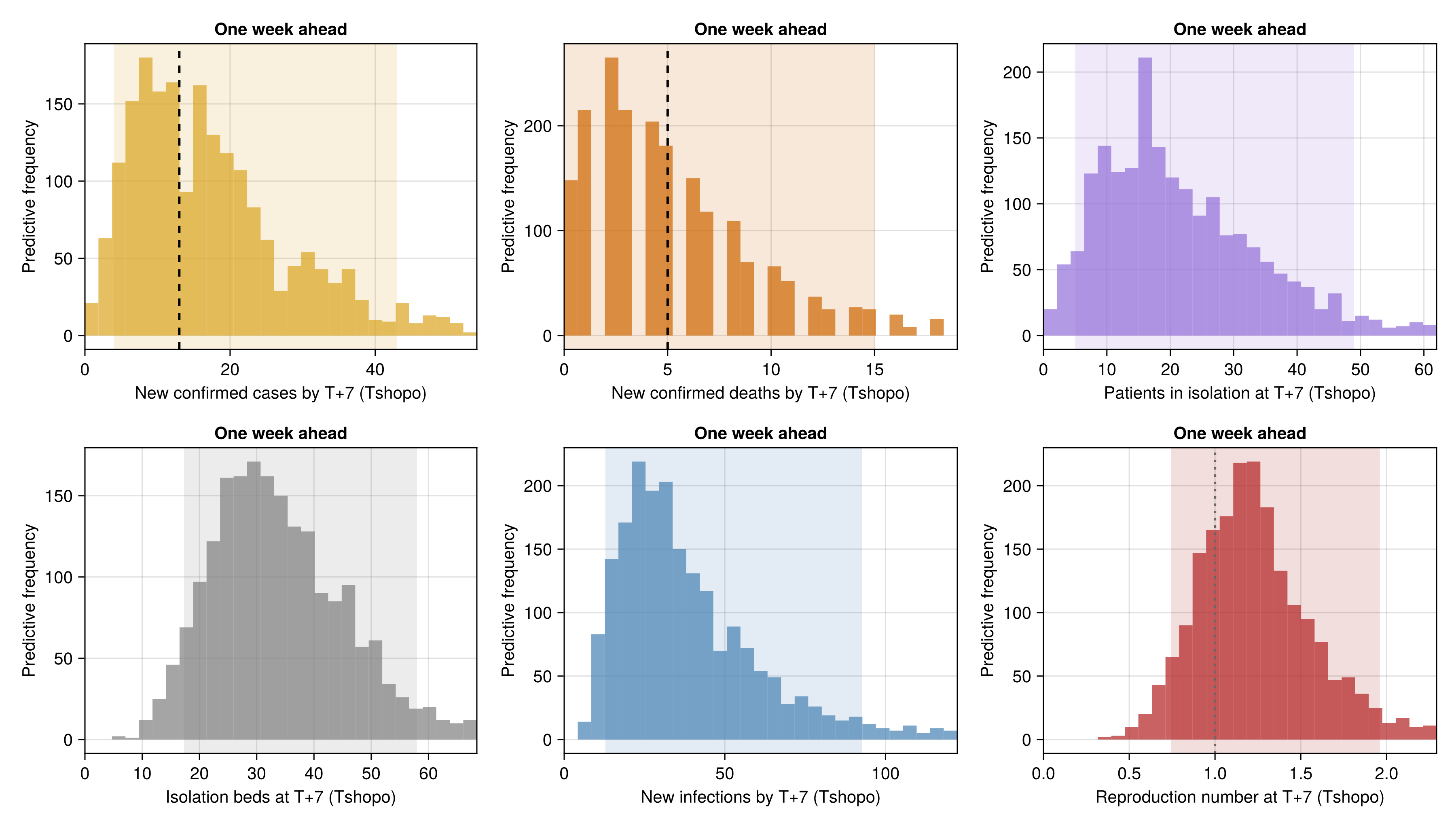
Tshopo	4–43	0–15	5–49	17–58	13–93	0.74–1.96	75%
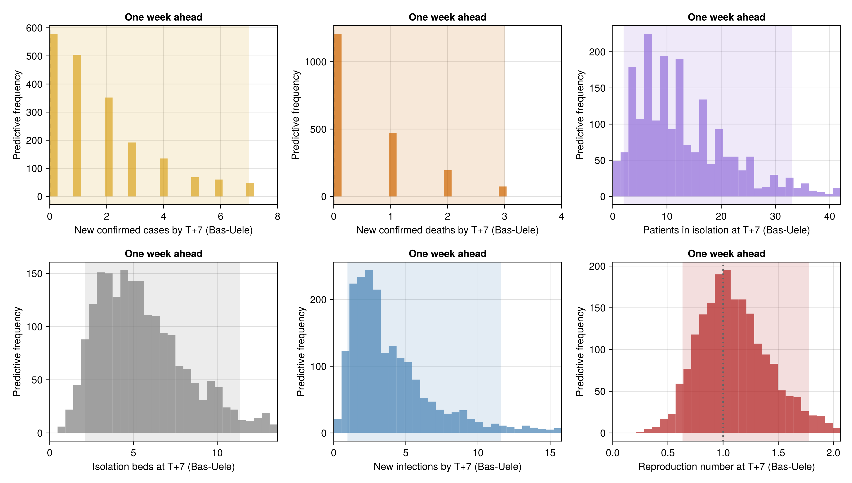
Bas-Uele	0–7	0–3	2–33	2–11	1–12	0.63–1.78	60%
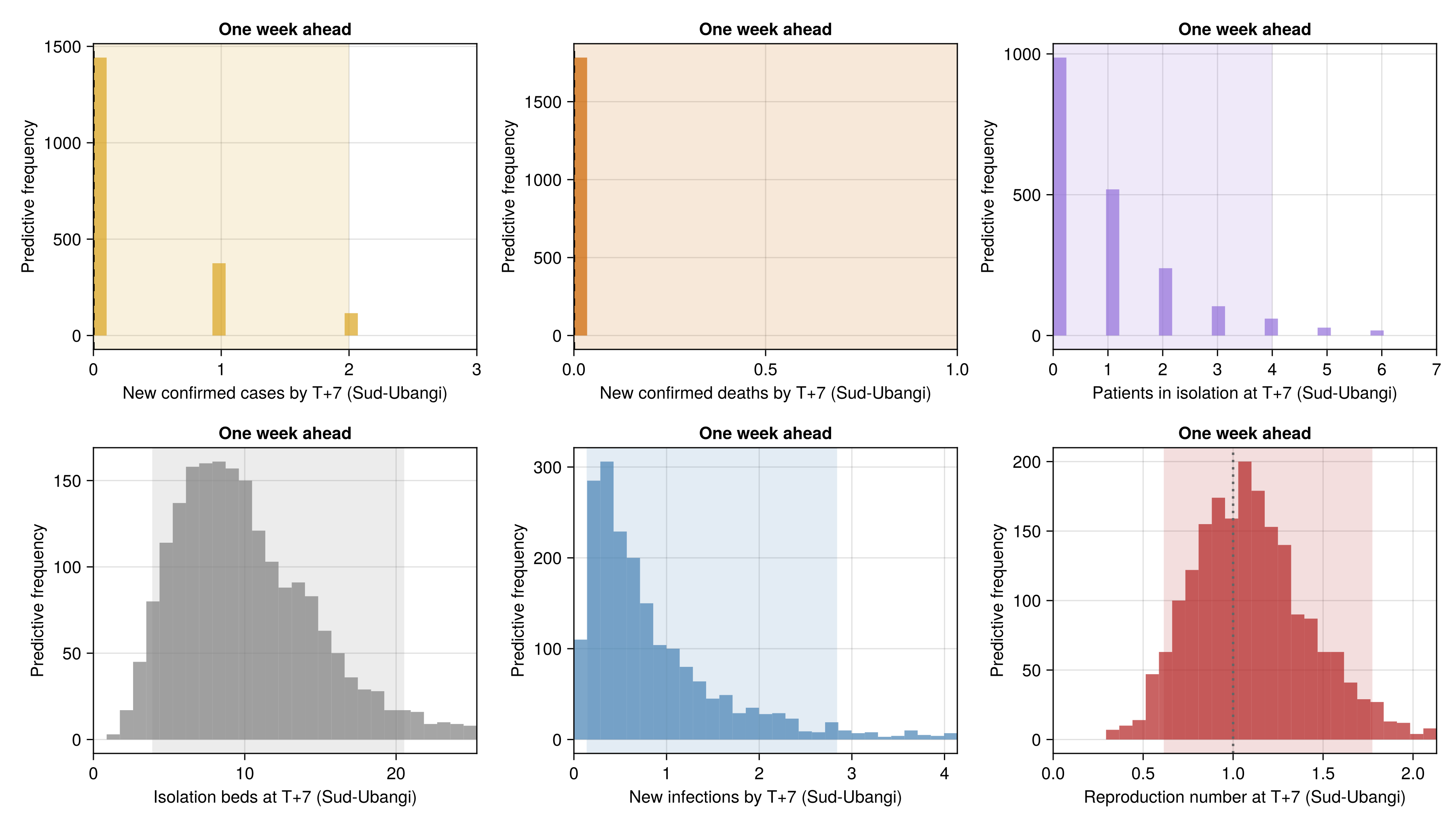
Sud-Ubangi	0–2	0–1	0–4	4–21	0–3	0.61–1.77	61%
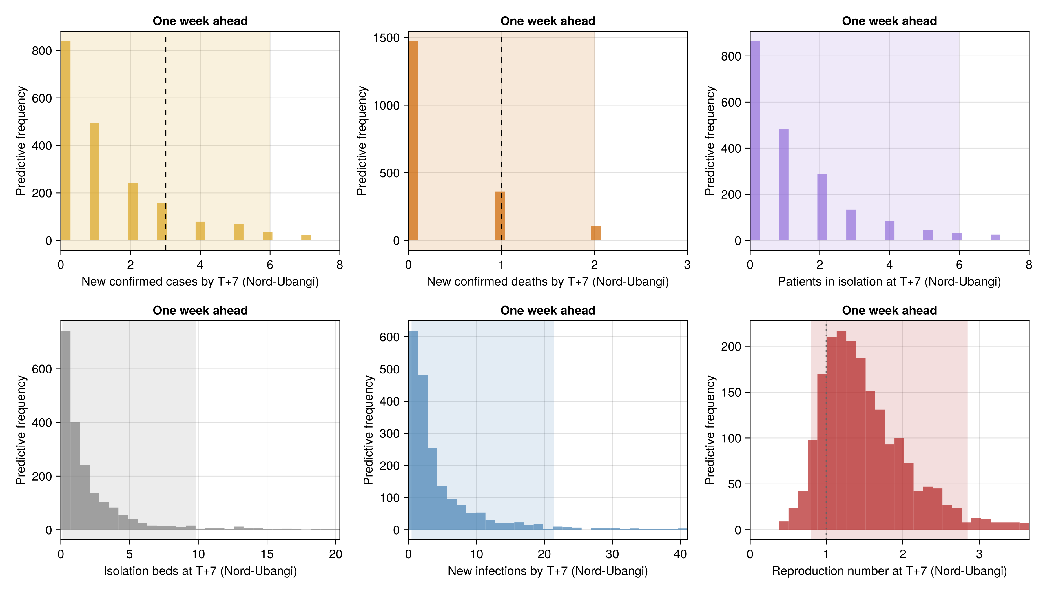
Nord-Ubangi	0–6	0–2	0–6	0–10	0–21	0.8–2.85	84%

Most new confirmed cases: Ituri, with probability 80%.
Most new confirmed deaths: Ituri, with probability 63%.
Growing at T+7: 7 of 8 provinces are more likely than not to be growing (Ituri, Nord-Kivu, Haut-Uele, Tshopo, Bas-Uele, Sud-Ubangi, Nord-Ubangi).
Beds full at T+7: Nord-Kivu, Bas-Uele are more likely than not to be at or above its beds.

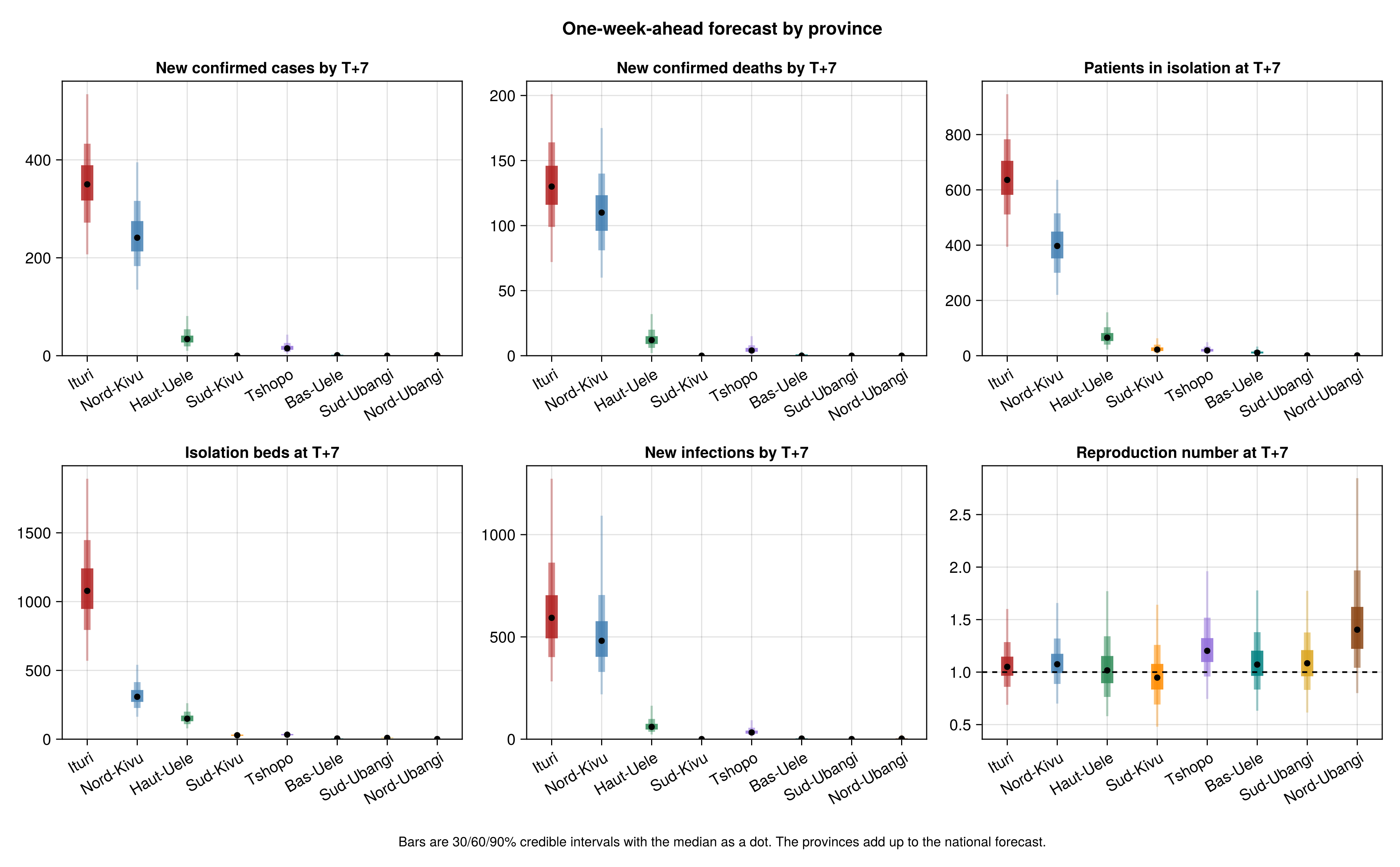
One-week-ahead forecast by province

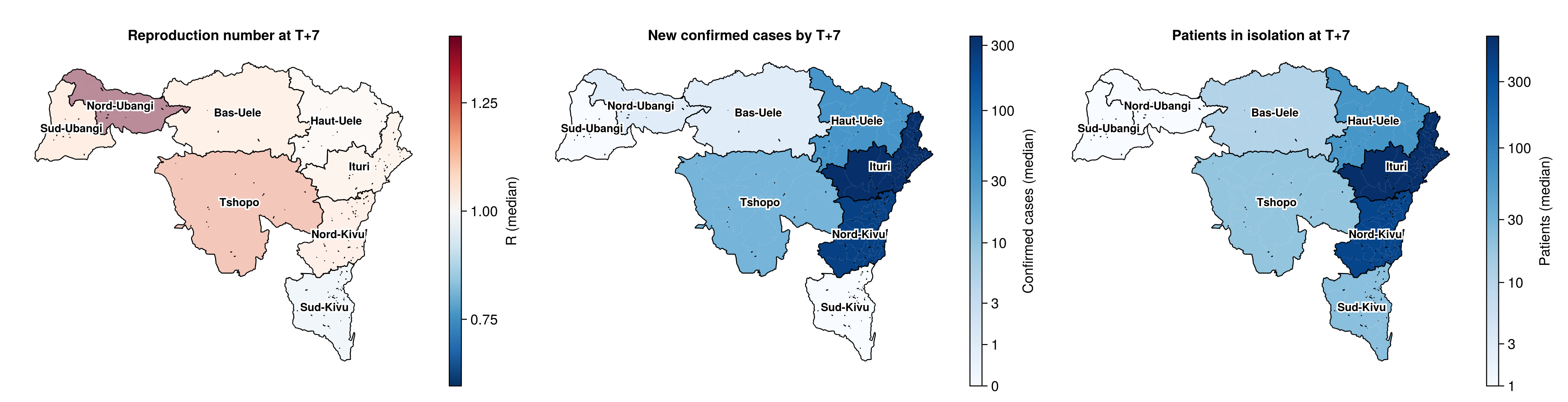
Each panel is one forecast target for the week after the cut-off, with the provinces side by side.

Build the forecast maps

julia

province_forecast_draws(col) = [
    float.(province_projection[province_projection.patch .== p, col])
        for p in 1:N_PATCHES
]
province_forecast_map = plot_province_map(
    filter(
        !isnothing,
        [
            (;
                province_map_summary(province_forecast_draws(:rt_forecast))...,
                title = "Reproduction number at T+7", diverging_at = 1.0,
                colorbar_label = "R (median)",
            ),
            (;
                values = province_map_summary(
                    province_forecast_draws(:confirmed_new)
                ).values,
                title = "New confirmed cases by T+7",
                scale = CairoMakie.Makie.pseudolog10,
                colorbar_label = "Confirmed cases (median)",
            ),
            :isolation_level in propertynames(province_projection) ? (;
                    values = province_map_summary(
                        province_forecast_draws(:isolation_level)
                    ).values,
                    title = "Patients in isolation at T+7",
                    scale = CairoMakie.Makie.pseudolog10,
                    colorbar_label = "Patients (median)",
                ) : nothing,
        ]
    )
);

Each province is shaded by its forecast. The reproduction number is centred on one, and a province whose 90% predictive interval spans one is washed out.

Province	Quantity	Lower 90%	Lower 60%	Lower 30%	Upper 30%	Upper 60%	Upper 90%
Ituri	New confirmed cases by T+7	207	272	317	389	433	534
Ituri	New confirmed deaths by T+7	72	99	116	146	164	201
Ituri	Patients in isolation at T+7	394	511	582	705	783	946
Ituri	Isolation beds at T+7	570	794	947	1242	1447	1893
Ituri	New infections by T+7	282	401	493	704	863	1273
Ituri	Reproduction number at T+7	0.69	0.86	0.97	1.15	1.29	1.6
Nord-Kivu	New confirmed cases by T+7	135	183	213	275	316	395
Nord-Kivu	New confirmed deaths by T+7	60	81	96	123	140	175
Nord-Kivu	Patients in isolation at T+7	220	300	352	449	515	636
Nord-Kivu	Isolation beds at T+7	163	227	271	357	415	541
Nord-Kivu	New infections by T+7	219	329	403	577	705	1093
Nord-Kivu	Reproduction number at T+7	0.7	0.89	0.99	1.17	1.32	1.66
Haut-Uele	New confirmed cases by T+7	10	19	27	41	54	81
Haut-Uele	New confirmed deaths by T+7	2	6	9	15	20	32
Haut-Uele	Patients in isolation at T+7	22	40	53	82	103	157
Haut-Uele	Isolation beds at T+7	78	109	131	171	200	261
Haut-Uele	New infections by T+7	23	36	47	75	99	164
Haut-Uele	Reproduction number at T+7	0.58	0.76	0.89	1.15	1.34	1.77
Sud-Kivu	New confirmed cases by T+7	0	0	0	0	0	2
Sud-Kivu	New confirmed deaths by T+7	0	0	0	0	0	1
Sud-Kivu	Patients in isolation at T+7	6	12	17	30	40	63
Sud-Kivu	Isolation beds at T+7	15	21	25	33	39	52
Sud-Kivu	New infections by T+7	0	0	0	1	1	2
Sud-Kivu	Reproduction number at T+7	0.48	0.69	0.83	1.08	1.26	1.64
Tshopo	New confirmed cases by T+7	4	8	12	20	26	43
Tshopo	New confirmed deaths by T+7	0	2	3	6	8	15
Tshopo	Patients in isolation at T+7	5	10	15	24	33	49
Tshopo	Isolation beds at T+7	17	24	28	37	44	58
Tshopo	New infections by T+7	13	21	27	42	56	93
Tshopo	Reproduction number at T+7	0.74	0.96	1.1	1.32	1.52	1.96
Bas-Uele	New confirmed cases by T+7	0	0	1	2	3	7
Bas-Uele	New confirmed deaths by T+7	0	0	0	1	1	3
Bas-Uele	Patients in isolation at T+7	2	6	8	15	20	33
Bas-Uele	Isolation beds at T+7	2	3	4	6	8	11
Bas-Uele	New infections by T+7	1	2	2	4	6	12
Bas-Uele	Reproduction number at T+7	0.63	0.83	0.96	1.2	1.38	1.78
Sud-Ubangi	New confirmed cases by T+7	0	0	0	0	1	2
Sud-Ubangi	New confirmed deaths by T+7	0	0	0	0	0	1
Sud-Ubangi	Patients in isolation at T+7	0	0	0	1	2	4
Sud-Ubangi	Isolation beds at T+7	4	6	8	11	14	21
Sud-Ubangi	New infections by T+7	0	0	0	1	1	3
Sud-Ubangi	Reproduction number at T+7	0.61	0.83	0.96	1.21	1.38	1.77
Nord-Ubangi	New confirmed cases by T+7	0	0	0	1	3	6
Nord-Ubangi	New confirmed deaths by T+7	0	0	0	0	1	2
Nord-Ubangi	Patients in isolation at T+7	0	0	0	1	2	6
Nord-Ubangi	Isolation beds at T+7	0	0	1	2	3	10
Nord-Ubangi	New infections by T+7	0	1	2	4	7	21
Nord-Ubangi	Reproduction number at T+7	0.8	1.04	1.22	1.62	1.97	2.85

Forecast for each province

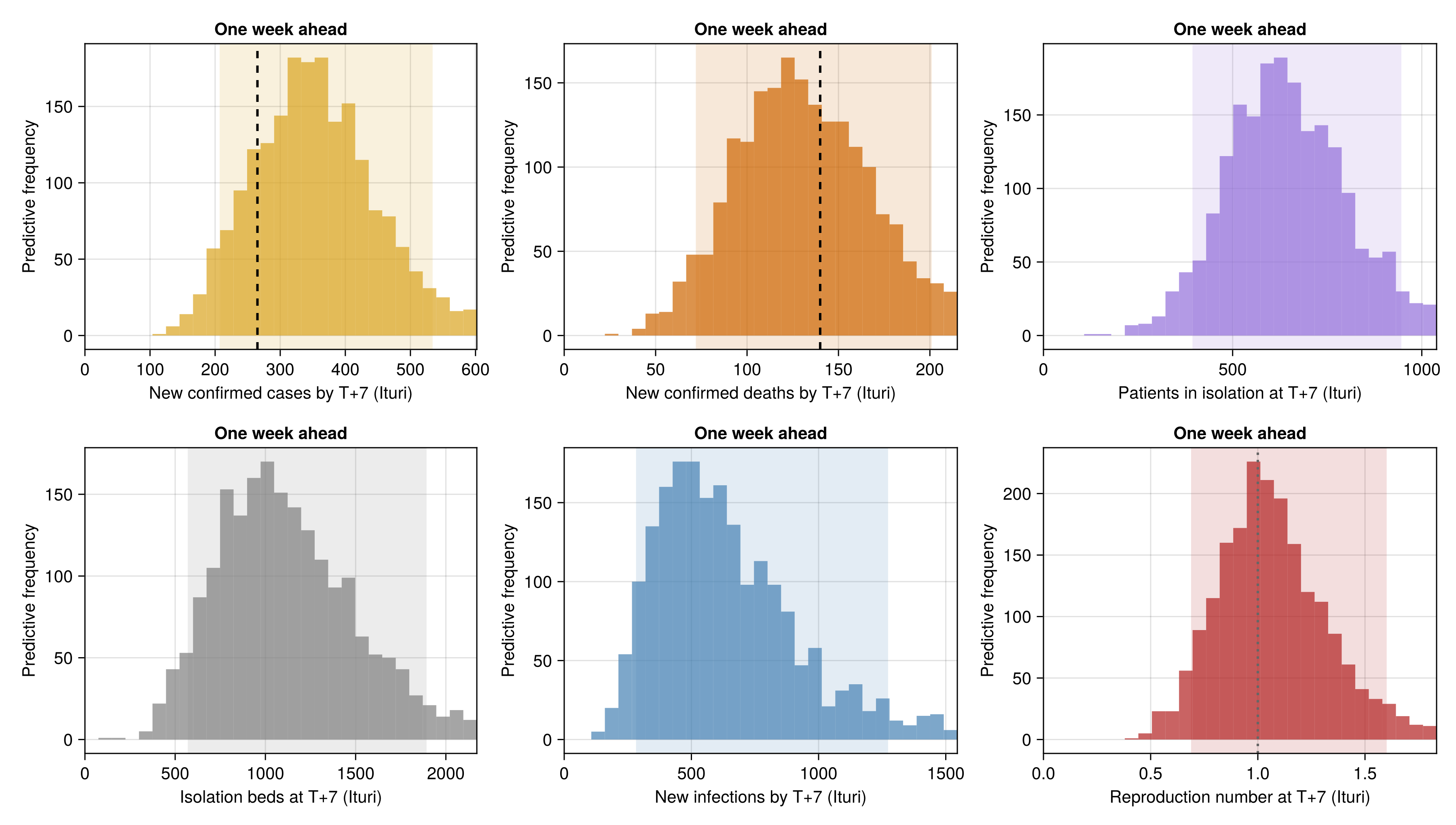
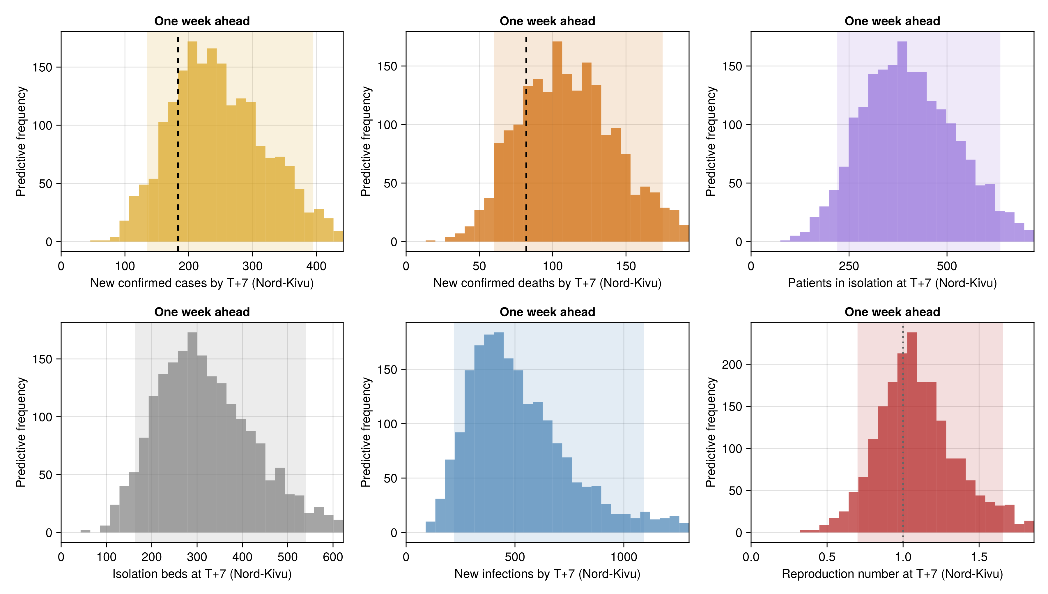
Each province's figure has one histogram per target with its 90% predictive interval shaded. The dashed rule on the case and death panels is the count the province reported over its most recent week.

Build the per-province figures

julia

# The spatial tables' most recent week in each province, clamped as the
# compositions are, so a downward revision reads as no new cases.
recent_cases = province_recent_counts(
    obs.province_confirmed_history, PROVINCE_NAMES, N_PATCHES
)
recent_deaths = province_recent_counts(
    obs.province_death_history, PROVINCE_NAMES, N_PATCHES
)
function forecast_province_observed(p)
    o = (;)
    recent_cases === nothing ||
        (o = merge(o, (; confirmed_new = recent_cases.counts[p])))
    recent_deaths === nothing ||
        (o = merge(o, (; confirmed_deaths_new = recent_deaths.counts[p])))
    return o
end
forecast_province_fig(p) = plot_province_forecast_detail(
    province_draws, province_projection;
    province = p, n_patches = N_PATCHES,
    observed = forecast_province_observed(p)
)
# The province blocks below are written out one per patch.
@assert N_PATCHES == 8 && PROVINCE_LABELS[1:8] == [
    "Ituri", "Nord-Kivu", "Haut-Uele",
    "Sud-Kivu", "Tshopo", "Bas-Uele", "Sud-Ubangi", "Nord-Ubangi",
]
# Cases and deaths come from separate tables, so each stream's observed
# week is stated on its own.
function forecast_province_recent_week(r, stream)
    r === nothing &&
        return "The spatial tables carry no recent week of $(stream)."
    return string(
        "The observed week of $(stream) runs from ",
        grid_date(r.start_day), " to ", grid_date(r.last_day), "."
    )
end
recent_note = join(
    [
        forecast_province_recent_week(recent_cases, "confirmed cases"),
        forecast_province_recent_week(recent_deaths, "confirmed deaths"),
        "Each ends at its last spatial vintage, which can be earlier than " *
            "the cut-off.",
    ], " "
);

The observed week of confirmed cases runs from 2026-10-13 to 2026-10-20. The observed week of confirmed deaths runs from 2026-10-13 to 2026-10-20. Each ends at its last spatial vintage, which can be earlier than the cut-off.

Ituri

Nord-Kivu

Haut-Uele

Sud-Kivu

Tshopo

Bas-Uele

Sud-Ubangi

Nord-Ubangi

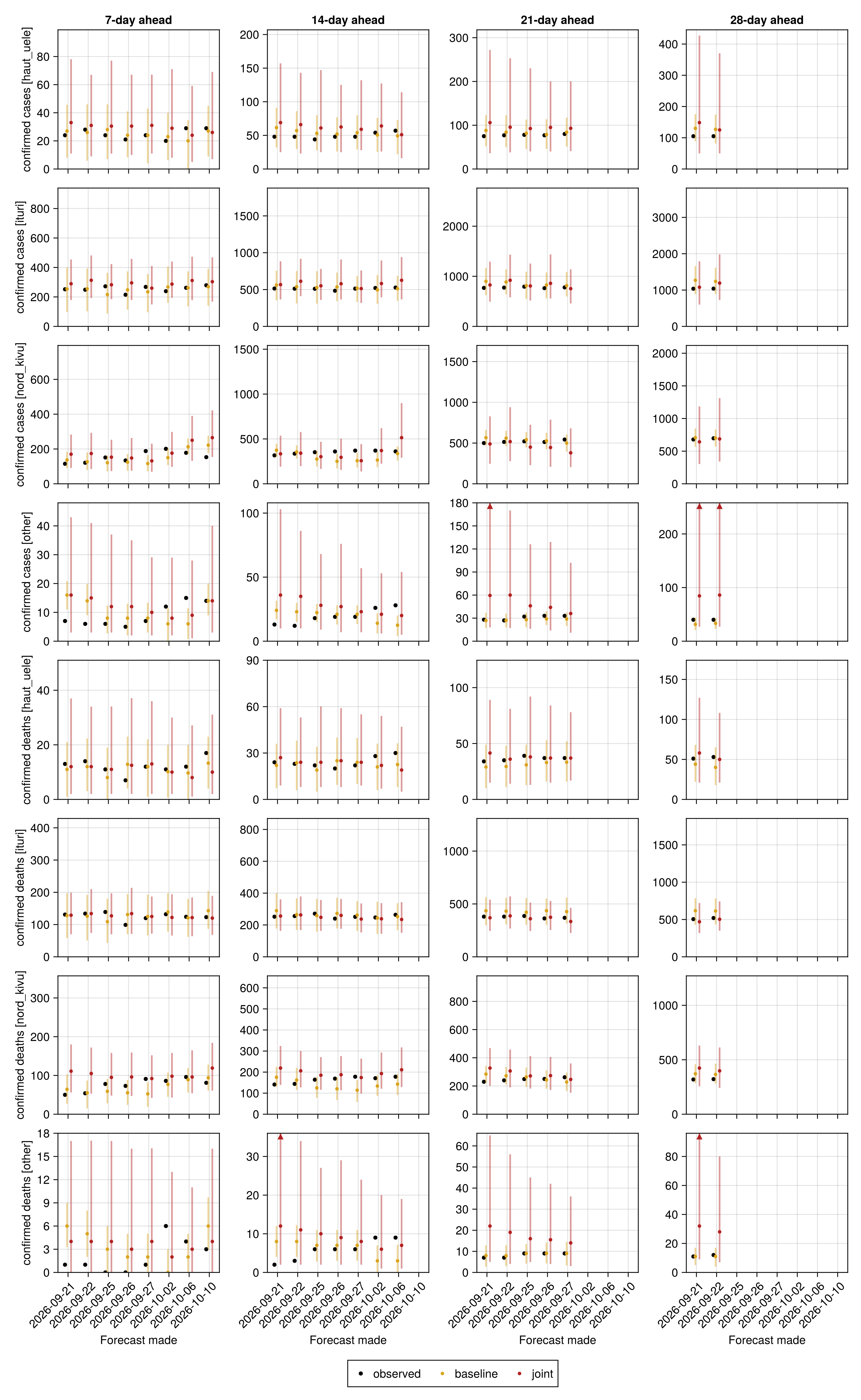
Past forecasts against what was observed

Load the archived province forecasts and their outcomes

julia

# Written by `scripts/score_releases.jl` from each release's
# `province_forecast.csv`, in the national overlay's schema. A missing
# file reads as an empty table, which the figure reports as nothing scored.
province_overlay_df = _release_data(
    joinpath("province", "forecast_overlay.csv"),
    (;
        release = String, made_date = Date, stream = String, horizon = Int,
        target_date = Date, fit = String, observed = Float64,
        median = Float64, lo30 = Float64, hi30 = Float64, lo60 = Float64,
        hi60 = Float64, lo90 = Float64, hi90 = Float64,
    )
)
province_overlay_fig = plot_forecast_overlay(
    scored_overlay(province_overlay_df);
    empty_message = "No projection forecast has been scored yet. " *
        "This fills in as releases accumulate."
);

Past province forecasts by the cut-off each was made from, one panel per stream and horizon, filling in as releases accumulate. Each shows its median and 90% predictive interval beside the persistence baseline and the count the province went on to report. A window holding a harmonisation-break day is left out, because that day's backfill is published for the country and not by province.

Saving province map assets

The dashboard map's province layer and its detail column read the per-province and national estimates and time series written here.

Write the province map estimates and time series

julia

# The national row reads the joint's national reproduction number and
# case-fatality ratio and the provinces' summed forecasts, patients in
# isolation and beds.
province_map_dir = joinpath(
    pkgdir(BVDOutbreakSize), "docs", "src", "summary_assets"
)
mkpath(province_map_dir)
has_death_forecast = :confirmed_deaths_new in propertynames(province_projection)
has_care_forecast = :isolation_level in propertynames(province_projection) &&
    :bed_capacity in propertynames(province_projection)
has_care = BVDOutbreakSize._has_key(chn_joint, :province_bed_capacity)
# Patients in isolation over beds, draw by draw.
care_ratio(iso, beds) = [i ./ b for (i, b) in zip(iso, beds)]
province_care_forecast = has_care_forecast ? (;
        isolation_forecast = province_forecast_draws(:isolation_level),
        beds_forecast = province_forecast_draws(:bed_capacity),
        bed_use_forecast = care_ratio(
            province_forecast_draws(:isolation_level),
            province_forecast_draws(:bed_capacity)
        ),
    ) : (;)
CSV.write(
    joinpath(province_map_dir, "province_estimates.csv"),
    province_map_estimates(
        chn_joint, province_forecast_draws(:confirmed_new);
        n_patches = N_PATCHES,
        deaths_forecast = has_death_forecast ?
            province_forecast_draws(:confirmed_deaths_new) : nothing,
        confirmed_history = obs.province_confirmed_history,
        death_history = obs.province_death_history, cutoff = obs.cutoff,
        isolation_history = obs.province_isolation_history,
        bed_history = obs.province_bed_capacity_history, n = obs.n,
        province_care_forecast...
    )
);
national_forecast_draws(col) = let d = province_projection
    [float(sum(d[d.draw .== i, col])) for i in sort(unique(d.draw))]
end
# The provinces' cut-off draws summed into one national draw vector.
national_care_draws(key) = let v = BVDOutbreakSize._per_patch(
        chn_joint, key, N_PATCHES
    )
    [sum(x[i] for x in v) for i in eachindex(first(v))]
end
national_care = has_care ? (;
        isolation = [national_care_draws(:province_expected_isolation)],
        beds = [national_care_draws(:province_bed_capacity)],
        bed_use = care_ratio(
            [national_care_draws(:province_expected_isolation)],
            [national_care_draws(:province_bed_capacity)]
        ),
    ) : (;)
national_care_forecast = has_care_forecast ? (;
        isolation_forecast = [national_forecast_draws(:isolation_level)],
        beds_forecast = [national_forecast_draws(:bed_capacity)],
        bed_use_forecast = care_ratio(
            [national_forecast_draws(:isolation_level)],
            [national_forecast_draws(:bed_capacity)]
        ),
    ) : (;)
CSV.write(
    joinpath(province_map_dir, "national_estimates.csv"),
    province_map_estimates(
        [vec(Array(chn_joint[:R_T]))],
        [national_forecast_draws(:confirmed_new)];
        deaths_forecast = has_death_forecast ?
            [national_forecast_draws(:confirmed_deaths_new)] : nothing,
        cfr = [vec(Array(chn_joint[:CFR]))],
        confirmed_history = Dict("national" => obs.confirmed_history),
        death_history = Dict("national" => obs.confirmed_deaths_history),
        cutoff = obs.cutoff, patch_names = ["national"],
        patch_labels = ["National"],
        members = Dict("national" => ["national"]),
        isolation_history = Dict("national" => obs.isolation_history),
        bed_history = Dict("national" => obs.bed_capacity_history),
        n = obs.n, national_care..., national_care_forecast...
    )
);
# The daily reproduction number and the weekly confirmed cases and deaths
# of each patch and of the country, keyed by the patch label, and the
# reported patients in isolation and beds over the same eight weeks, keyed
# by source province.
province_ts_rt_args = (;
    n = obs.n, breakpoint = _BREAKPOINT, rt_start = _rt_start_plot,
    rt_walk_start = clamp(_BREAKPOINT - RT_WALK_LEAD, _rt_start_plot, obs.n),
    ramp = RT_INTERVENTION_RAMP,
)
province_ts_inc = province_increment_matrix(
    obs.province_confirmed_history, PROVINCE_NAMES, N_PATCHES
)
province_ts_deaths = province_increment_matrix(
    obs.province_death_history, PROVINCE_NAMES, N_PATCHES
)
national_increments(c) = isempty(c) ? zeros(Int, 1, 0) :
    reshape([c[1]; max.(diff(c), 0)], 1, :)
# Each patch's and the country's weekly counts from their increments.
function province_weekly(inc, national)
    return vcat(
        weekly_count_table(
            inc.days, inc.increments, PROVINCE_LABELS[1:N_PATCHES];
            cutoff = obs.cutoff, n = obs.n
        ),
        weekly_count_table(
            national.days, national_increments(national.counts),
            ["National"]; cutoff = obs.cutoff, n = obs.n
        )
    )
end
# Tag a long table with the series it holds.
_with_series(t, s) = (t[!, :series] .= s; t)
CSV.write(
    joinpath(province_map_dir, "province_timeseries.csv"),
    vcat(
        _with_series(
            rt_quantile_table(
                [
                    reconstruct_patch_rt(
                        chn_joint; n_patches = N_PATCHES,
                        province_ts_rt_args...
                    );
                    [reconstruct_rt(chn_joint; province_ts_rt_args...)]
                ],
                [PROVINCE_LABELS[1:N_PATCHES]; "National"];
                cutoff = obs.cutoff, n = obs.n, from = _rt_start_plot
            ), "rt"
        ),
        _with_series(
            province_weekly(province_ts_inc, obs.confirmed_history), "cases"
        ),
        _with_series(
            province_weekly(province_ts_deaths, obs.confirmed_deaths_history),
            "deaths"
        ),
        _with_series(
            reported_level_table(
                merge(
                    obs.province_isolation_history,
                    Dict("National" => obs.isolation_history)
                ); cutoff = obs.cutoff, n = obs.n, from = obs.n - 55
            ), "isolation"
        ),
        _with_series(
            reported_level_table(
                merge(
                    obs.province_bed_capacity_history,
                    Dict("National" => obs.bed_capacity_history)
                ); cutoff = obs.cutoff, n = obs.n, from = obs.n - 55
            ), "beds"
        );
        cols = :union
    )
);
# The same three tables into the release outputs, so each results release
# carries the dashboard map's province and national inputs at its cut-off.
output_dir = get(
    ENV, "BVD_OUTPUT_DIR",
    joinpath(pkgdir(BVDOutbreakSize), "output")
)
mkpath(output_dir)
for f in (
        "province_estimates.csv", "national_estimates.csv",
        "province_timeseries.csv",
    )
    cp(joinpath(province_map_dir, f), joinpath(output_dir, f); force = true)
end

The full analysis code, data and model definitions are in the epiforecasts/BVDOutbreakSize repository.

Province forecasts ​

Summary ​

One-week-ahead forecast by province ​

Forecast for each province ​

Ituri ​

Nord-Kivu ​

Haut-Uele ​

Sud-Kivu ​

Tshopo ​

Bas-Uele ​

Sud-Ubangi ​

Nord-Ubangi ​

Past forecasts against what was observed ​

Saving province map assets ​

Province forecasts

Summary

One-week-ahead forecast by province

Forecast for each province

Ituri

Nord-Kivu

Haut-Uele

Sud-Kivu

Tshopo

Bas-Uele

Sud-Ubangi

Nord-Ubangi

Past forecasts against what was observed

Saving province map assets