Prior choice and specification guide

Introduction

This vignette provides practical guidance on specifying and choosing priors for EpiNow2 models. While the package provides sensible defaults for all priors, understanding when and how to modify them can improve model performance for your specific application.

This guide covers priors for the three main modelling functions:

estimate_infections() (renewal equation and non-mechanistic models)
estimate_secondary() (secondary observations like deaths or hospitalizations)
estimate_truncation() (truncation distribution estimation)

What this guide covers:

A comprehensive table of all priors in EpiNow2
The expected impact of different prior choices
Guidance on when to change defaults
Practical examples of prior specification

What this guide does NOT cover:

Mathematical derivations (see Model definition)
Technical implementation details (see Gaussian Process implementation details)
General Bayesian prior elicitation theory (see the Stan Prior Choice Recommendations)

Key principle: All defaults in EpiNow2 aim to provide sensible defaults that work across a range of pathogens and settings. For a specific application with domain knowledge, you may benefit from more informative priors.

Important default: The default generation time is Fixed(1), meaning all transmission occurs after 1 day. With this default, $R_t$ represents the daily exponential growth rate rather than the traditional reproduction number. For epidemiologically meaningful $R_t$ estimates, you should always specify a realistic generation time distribution from the literature (see Generation time distribution).

Set up

We load the EpiNow2 package and the posterior and data.table packages which we will use for convergence diagnostics and data wrangling, respectively.

library(EpiNow2)
#> 
#> Attaching package: 'EpiNow2'
#> The following object is masked from 'package:stats':
#> 
#>     Gamma
library(posterior)
#> This is posterior version 1.6.1
#> 
#> Attaching package: 'posterior'
#> The following objects are masked from 'package:stats':
#> 
#>     mad, sd, var
#> The following objects are masked from 'package:base':
#> 
#>     %in%, match
library(data.table)

We also set up example data and parameters that will be used in code examples throughout this vignette.

# Example data for estimate_infections
reported_cases <- example_confirmed[1:60]

# Example data for estimate_secondary
secondary_data <- copy(example_confirmed)[1:60]
setnames(secondary_data, "confirm", "primary")
secondary_data[, scaling := 0.4]
secondary_data[, meanlog := 1.8][, sdlog := 0.5]
secondary_data <- convolve_and_scale(secondary_data, type = "incidence")

# Example data for estimate_truncation
truncation_data <- example_truncated

# Example delays
reporting_delay <- LogNormal(mean = 2, sd = 1, max = 10)
delay <- example_incubation_period + reporting_delay

# Fast Stan settings for vignette building
# (Use default settings for actual analyses)
stan <- stan_opts(
  samples = 100,
  warmup = 100,
  chains = 2,
  control = list(adapt_delta = 0.9)
)

Overview of all priors

The following tables list all priors available in EpiNow2, organised by modelling function.

estimate_infections() priors

estimate_infections() supports two models: renewal equation (default) and non-mechanistic/deconvolution.

Component	Model	Function	Parameter	Default	Notes
Reproduction number (Rt)
Initial R₀ / mean Rt	Renewal only	`rt_opts()`	`prior`	`LogNormal(mean = 1, sd = 1)`	When choosing `gp_on = "R0"`, reverts to this when no data
Random walk
Step size SD	Renewal only	`rt_opts()`	`rw`	`HalfNormal(0, 0.1)`	Set step size via `rw` argument
Gaussian Process
Length scale	Both	`gp_opts()`	`ls`	`LogNormal(mean = 21, sd = 7, max = 60)`	Controls smoothness over time
Magnitude	Both	`gp_opts()`	`alpha`	`Normal(mean = 0, sd = 0.01)`	Controls amplitude of variations
Back-calculation
Prior source	Non-mechanistic only	`backcalc_opts()`	`prior`	`"reports"`	Options: “reports”, “infections”, “none”
Observation model
Overdispersion	Both	`obs_opts()`	`dispersion`	`Normal(mean = 0, sd = 0.25)`	1/√φ parameterisation
Scaling	Both	`obs_opts()`	`scale`	`Fixed(1)`	Ascertainment rate
Day of week	Both	(internal)	(auto)	`Dirichlet(1, ..., 1)`	Turn off via `week_effect = FALSE`
Generation time
Parameters	Renewal only	`gt_opts()`	`dist`	`Fixed(1)`	Default: Rt is daily exponential growth rate
Delays
Parameters	Both	`delay_opts()`	`dist`	`Fixed(0)`	No delay by default
Truncation
Distribution	Both	`trunc_opts()`	`dist`	`Fixed(0)`	No truncation by default

estimate_secondary() priors

Component	Function	Parameter	Default	Notes
Delays (primary to secondary)
Parameters	`delay_opts()`	`dist`	`LogNormal(meanlog = Normal(2.5, 0.5), sdlog = Normal(0.47, 0.25), max = 30)`	Time from primary to secondary event
Observation model
Scaling	`obs_opts()`	`scale`	`Fixed(1)`	Fraction of primary events leading to secondary
Overdispersion	`obs_opts()`	`dispersion`	`Normal(mean = 0, sd = 0.25)`	1/√φ parameterisation
Day of week	(internal)	(auto)	`Dirichlet(1, ..., 1)`	Turn off via `week_effect = FALSE`

estimate_truncation() priors

Component	Function	Parameter	Default	Notes
Truncation distribution
Parameters	`trunc_opts()`	`dist`	`LogNormal(meanlog = Normal(0, 1), sdlog = Normal(1, 1), max = 10)`	Describes reporting delays
Observation model
Overdispersion	(internal)	(auto)	`HalfNormal(0, 1)`	1/√φ parameterisation; not directly adjustable
Noise term	(internal)	(auto)	`HalfNormal(0, 1)`	Not directly adjustable

Prior impacts and choice guidance

This section explains what effects you can expect from modifying each prior, and when you might want to do so.

Reproduction number

What it controls: The prior distribution for the reproduction number. Its role depends on the Gaussian Process specification:

Differenced GP (default, gp_on = "R_t-1"): This is the prior for $R_0$ at the start of the time series. When there is no data (e.g., early in the time series before the seeding period ends, or when doing real-time estimates of delayed quantities), $R_t$ reverts to the last estimated value but with expanding uncertainty as the zero-centered GP of differences continues.
Stationary GP (gp_on = "R0"): This is the prior mean that $R_t$ reverts to throughout the time series when there is no data (e.g., early in the time series, or near the present when there are delays). Useful when you want estimates of $R_t$ to return to a baseline value in the absence of information.

Default: LogNormal(mean = 1, sd = 1)

This default corresponds to a median of 1 (range 0.4 to 2.7 at 95% prior probability), centred on the epidemic threshold.

Expected impact of changes:

Tighter prior (smaller sd): Speeds up MCMC convergence if your prior is accurate, but may bias estimates if wrong. Use when you have strong prior knowledge about $R_0$ for your pathogen.
Higher mean: Shifts the initial $R_0$ estimate upward (differenced) or provides a higher reversion point (stationary). Use for fast-spreading pathogens based on prior knowledge from the literature.
Wider prior (larger sd): More flexible but may lead to slower convergence and/or identifiability problems. Use when very uncertain about initial dynamics.

When to modify:

You have reliable estimates from similar outbreaks or the literature
You’re analysing a well-characterised pathogen (e.g., influenza pandemic with $R_0$ typically 1.5-2.5, or emerging outbreaks of measles in immunologically naive populations)
Using stationary GP and want a specific baseline for $R_t$ to revert to

Example:

# For a measles outbreak with strong prior knowledge
rt_opts(prior = LogNormal(mean = 15, sd = 2))
#> $use_rt
#> [1] TRUE
#> 
#> $rw
#> [1] 0
#> 
#> $use_breakpoints
#> [1] TRUE
#> 
#> $future
#> [1] "latest"
#> 
#> $gp_on
#> [1] "R_t-1"
#> 
#> $pop_period
#> [1] "forecast"
#> 
#> $pop_floor
#> [1] 1
#> 
#> $growth_method
#> [1] "infections"
#> 
#> $pop
#> - fixed value:
#>   0
#> 
#> $prior
#> - lognormal distribution:
#>   meanlog:
#>     2.7
#>   sdlog:
#>     0.13
#> 
#> attr(,"class")
#> [1] "rt_opts" "list"

# For uncertain but likely growing outbreak
rt_opts(prior = LogNormal(mean = 2, sd = 1))
#> $use_rt
#> [1] TRUE
#> 
#> $rw
#> [1] 0
#> 
#> $use_breakpoints
#> [1] TRUE
#> 
#> $future
#> [1] "latest"
#> 
#> $gp_on
#> [1] "R_t-1"
#> 
#> $pop_period
#> [1] "forecast"
#> 
#> $pop_floor
#> [1] 1
#> 
#> $growth_method
#> [1] "infections"
#> 
#> $pop
#> - fixed value:
#>   0
#> 
#> $prior
#> - lognormal distribution:
#>   meanlog:
#>     0.58
#>   sdlog:
#>     0.47
#> 
#> attr(,"class")
#> [1] "rt_opts" "list"

# Stationary GP reverting to R_t = 2 when no data
rt_opts(
  prior = LogNormal(mean = 2, sd = 0.5),
  gp_on = "R0"
)
#> $use_rt
#> [1] TRUE
#> 
#> $rw
#> [1] 0
#> 
#> $use_breakpoints
#> [1] TRUE
#> 
#> $future
#> [1] "latest"
#> 
#> $gp_on
#> [1] "R0"
#> 
#> $pop_period
#> [1] "forecast"
#> 
#> $pop_floor
#> [1] 1
#> 
#> $growth_method
#> [1] "infections"
#> 
#> $pop
#> - fixed value:
#>   0
#> 
#> $prior
#> - lognormal distribution:
#>   meanlog:
#>     0.66
#>   sdlog:
#>     0.25
#> 
#> attr(,"class")
#> [1] "rt_opts" "list"

Gaussian Process length scale

What it controls: The smoothness of changes in the reproduction number over time, measured in days. Larger values = smoother changes; smaller values = more rapid fluctuations.

Default: LogNormal(mean = 21, sd = 7, max = 60)

This corresponds to a median of 21 days (range 9 to 36 days at 95% prior probability), reflecting gradual changes typical of epidemics with interventions happening over weeks.

Expected impact of changes:

Shorter length scale (smaller mean): Allows $R_t$ to change more rapidly day-to-day. Results in less smooth $R_t$ estimates that can track sudden changes (e.g., lockdowns) more quickly. May overfit to noise if too short.
Longer length scale (larger mean): Forces smoother $R_t$ changes over time. More stable estimates but may miss rapid shifts in transmission. Can undersmooth if too long.
Wider uncertainty (larger sd): Lets the data determine the smoothness. More flexible but computationally expensive.

When to modify:

Shorter (mean ~7-14 days): When expecting rapid policy changes, modelling short outbreaks, or seeing sudden shifts in data
Longer (mean ~28+ days): When transmission changes gradually, in stable endemic settings, or with noisy data
Maximum adjustment: Set max lower if working with short time series (e.g., max=30 for 60-day outbreak)

Example:

# For outbreak with weekly policy changes
gp_opts(ls = LogNormal(mean = 7, sd = 3, max = 30))
#> $basis_prop
#> [1] 0.2
#> 
#> $boundary_scale
#> [1] 1.5
#> 
#> $ls
#> - lognormal distribution (max: 30):
#>   meanlog:
#>     1.9
#>   sdlog:
#>     0.41
#> 
#> $alpha
#> - normal distribution:
#>   mean:
#>     0
#>   sd:
#>     0.01
#> 
#> $kernel
#> [1] "matern"
#> 
#> $matern_order
#> [1] 1.5
#> 
#> $w0
#> [1] 1
#> 
#> attr(,"class")
#> [1] "gp_opts" "list"

# For gradually evolving endemic disease
gp_opts(ls = LogNormal(mean = 28, sd = 10, max = 90))
#> $basis_prop
#> [1] 0.2
#> 
#> $boundary_scale
#> [1] 1.5
#> 
#> $ls
#> - lognormal distribution (max: 90):
#>   meanlog:
#>     3.3
#>   sdlog:
#>     0.35
#> 
#> $alpha
#> - normal distribution:
#>   mean:
#>     0
#>   sd:
#>     0.01
#> 
#> $kernel
#> [1] "matern"
#> 
#> $matern_order
#> [1] 1.5
#> 
#> $w0
#> [1] 1
#> 
#> attr(,"class")
#> [1] "gp_opts" "list"

Gaussian Process magnitude

What it controls: The amplitude of variations in the Gaussian Process.

For renewal equation model: This controls variations in $\log(R_t)$ and is the prior standard deviation around the GP trend (stationary GP) or around zero (differenced GP).
For non-mechanistic model: This controls variations in log infections directly, and typically requires a less constrained prior since it scales with the infection level rather than $R_t$ .

Default: Normal(mean = 0, sd = 0.01)

For the renewal equation model, this corresponds to a half-normal (since negative values are truncated) with 95% of prior mass below 0.02, reflecting small changes in $\log(R_t)$ .

Expected impact of changes:

Larger sd (e.g., 0.05-0.1): Allows bigger jumps over time. Useful for outbreaks with large, real variations in transmission (e.g., due to major interventions) or for non-mechanistic models. May overfit if too large.
Smaller sd (e.g., 0.005): Constrains to change very gradually. Good for stable situations or very noisy data. May underfit real changes if too small.

When to modify:

Larger: Modelling outbreaks with major interventions (lockdowns, vaccination campaigns), high real variation, or using the non-mechanistic model
Smaller: Modelling stable endemic transmission or when data is very noisy relative to sample size
Note: The default works well for the renewal equation model in most scenarios, but may need adjustment for the non-mechanistic model

Example:

# For outbreak with major interventions
gp_opts(alpha = Normal(mean = 0, sd = 0.05))
#> $basis_prop
#> [1] 0.2
#> 
#> $boundary_scale
#> [1] 1.5
#> 
#> $ls
#> - lognormal distribution (max: 60):
#>   meanlog:
#>     3
#>   sdlog:
#>     0.32
#> 
#> $alpha
#> - normal distribution:
#>   mean:
#>     0
#>   sd:
#>     0.05
#> 
#> $kernel
#> [1] "matern"
#> 
#> $matern_order
#> [1] 1.5
#> 
#> $w0
#> [1] 1
#> 
#> attr(,"class")
#> [1] "gp_opts" "list"

# For very stable transmission
gp_opts(alpha = Normal(mean = 0, sd = 0.005))
#> $basis_prop
#> [1] 0.2
#> 
#> $boundary_scale
#> [1] 1.5
#> 
#> $ls
#> - lognormal distribution (max: 60):
#>   meanlog:
#>     3
#>   sdlog:
#>     0.32
#> 
#> $alpha
#> - normal distribution:
#>   mean:
#>     0
#>   sd:
#>     0.005
#> 
#> $kernel
#> [1] "matern"
#> 
#> $matern_order
#> [1] 1.5
#> 
#> $w0
#> [1] 1
#> 
#> attr(,"class")
#> [1] "gp_opts" "list"

Random walk for $R_t$ (alternative to GP)

What it controls: Step-wise changes in $R_t$ at fixed intervals instead of smooth GP changes.

Default: Not used (GP is default). When enabled via rt_opts(rw = 7), the prior SD is HalfNormal(0, 0.1).

Expected impact of changes:

Shorter steps (e.g., rw = 1): $R_t$ can change daily. Very flexible, like a short GP length scale. Fast to compute but may overfit.
Longer steps (e.g., rw = 7 or rw = 14): $R_t$ constant within each week/fortnight. Appropriate when transmission changes are discrete (policy changes) rather than continuous.

When to modify:

Use random walk instead of GP when you believe transmission changes are discrete rather than smooth
Use weekly (rw = 7) when transmission dynamics change at weekly intervals
Use daily (rw = 1) for maximum flexibility with fast computation (but risk overfitting)

Example:

# Weekly step changes
fit_rw <- estimate_infections(
  reported_cases,
  generation_time = gt_opts(example_generation_time),
  delays = delay_opts(delay),
  rt = rt_opts(prior = LogNormal(mean = 2, sd = 0.5), rw = 7),
  gp = NULL,  # Disable GP when using random walk
  stan = stan
)
#> Warning: The largest R-hat is NA, indicating chains have not mixed.
#> Running the chains for more iterations may help. See
#> https://mc-stan.org/misc/warnings.html#r-hat
#> Warning: Bulk Effective Samples Size (ESS) is too low, indicating posterior means and medians may be unreliable.
#> Running the chains for more iterations may help. See
#> https://mc-stan.org/misc/warnings.html#bulk-ess
#> Warning: Tail Effective Samples Size (ESS) is too low, indicating posterior variances and tail quantiles may be unreliable.
#> Running the chains for more iterations may help. See
#> https://mc-stan.org/misc/warnings.html#tail-ess

Observation model: overdispersion

What it controls: How much extra variability exists in reported cases beyond Poisson variation. The parameter is 1/√φ where φ is the negative binomial overdispersion.

Default: Normal(mean = 0, sd = 0.25)

With truncation at 0, this half-normal has 95% prior mass below 0.5, corresponding to moderate overdispersion.

Expected impact of changes:

Larger sd (e.g., 0.5-1.0): Allows for more overdispersion, meaning reported counts can be much more variable than a Poisson model. Use with highly variable reporting systems.
Smaller sd (e.g., 0.1): Tighter around Poisson variance. Use for high-quality surveillance with consistent reporting.
Change to Poisson: Set family = "poisson" in obs_opts(). Appropriate for large, stable counts with minimal extra variation.

When to modify:

More dispersed: Weekend effects, variable testing capacity, small outbreak counts, or low-resource settings
Less dispersed: Large outbreaks with stable reporting infrastructure
Switch to Poisson: Very large counts (>1000s daily) from stable reporting systems and when confident in model specification. Note that negative binomial overdispersion can absorb model misspecification, so switching to Poisson requires both high-quality data and confidence that the model structure is appropriate.

Example:

# For highly variable reporting
obs_opts(dispersion = Normal(mean = 0, sd = 0.5))
#> $family
#> [1] "negbin"
#> 
#> $dispersion
#> - normal distribution:
#>   mean:
#>     0
#>   sd:
#>     0.5
#> 
#> $weight
#> [1] 1
#> 
#> $week_effect
#> [1] TRUE
#> 
#> $week_length
#> [1] 7
#> 
#> $scale
#> - fixed value:
#>   1
#> 
#> $accumulate
#> [1] 0
#> 
#> $likelihood
#> [1] TRUE
#> 
#> $return_likelihood
#> [1] FALSE
#> 
#> $na_as_missing_default_used
#> [1] TRUE
#> 
#> attr(,"class")
#> [1] "obs_opts" "list"

# For stable, high-quality surveillance
obs_opts(family = "poisson")  # No dispersion parameter needed
#> $family
#> [1] "poisson"
#> 
#> $dispersion
#> - normal distribution:
#>   mean:
#>     0
#>   sd:
#>     0.25
#> 
#> $weight
#> [1] 1
#> 
#> $week_effect
#> [1] TRUE
#> 
#> $week_length
#> [1] 7
#> 
#> $scale
#> - fixed value:
#>   1
#> 
#> $accumulate
#> [1] 0
#> 
#> $likelihood
#> [1] TRUE
#> 
#> $return_likelihood
#> [1] FALSE
#> 
#> $na_as_missing_default_used
#> [1] TRUE
#> 
#> attr(,"class")
#> [1] "obs_opts" "list"

Observation model: scaling

What it controls: The scale parameter in obs_opts() is shared by both estimate_infections() and estimate_secondary(), but represents different quantities in each context:

For estimate_infections(): The proportion of infections that are ultimately reported (ascertainment rate)
For estimate_secondary(): The fraction of primary events leading to secondary events (e.g., case fatality rate, hospitalization rate)

Default: Fixed(1) for both functions

For estimate_infections(), this assumes all infections are reported. For estimate_secondary(), this assumes a 1:1 relationship between primary and secondary events (which is rarely realistic).

Expected impact of changes:

For estimate_infections():

Estimate scaling (e.g., Normal(mean=0.3, sd=0.1)): Allows model to estimate underreporting. Reported cases = scaling × latent infections × delay convolution. Useful when you know reporting is incomplete but don’t know the rate.
Fixed lower value (e.g., Fixed(0.5)): Assumes you know 50% are reported. Changes interpretation of infections but not $R_t$ .

For estimate_secondary():

Tight prior (e.g., Normal(mean=0.01, sd=0.005)): Constrains estimates near prior (e.g., 1% case fatality rate), faster convergence
Wide prior (e.g., Normal(mean=0.05, sd=0.05)): Flexible but may be poorly identified without long time series

When to modify:

For estimate_infections():

Nearly always keep at Fixed(1) and interpret “infections” as “reported infections”
Estimate only if: You have external data to anchor scale (seroprevalence, death rates) AND can set an informative prior on the ascertainment rate
Identifiability warning: Scaling and initial infections are weakly identified; estimating scale can cause convergence issues without strong external information

For estimate_secondary():

Always specify based on domain knowledge (unlike estimate_infections(), the default of 1 is rarely appropriate)
Use tighter priors with external estimates (e.g., infection fatality rate from serology studies)

Example:

# estimate_infections(): Estimating with informative prior from serology
obs_opts(scale = Normal(mean = 0.2, sd = 0.05, max = 1))
#> $family
#> [1] "negbin"
#> 
#> $dispersion
#> - normal distribution:
#>   mean:
#>     0
#>   sd:
#>     0.25
#> 
#> $weight
#> [1] 1
#> 
#> $week_effect
#> [1] TRUE
#> 
#> $week_length
#> [1] 7
#> 
#> $scale
#> - normal distribution (max: 1):
#>   mean:
#>     0.2
#>   sd:
#>     0.05
#> 
#> $accumulate
#> [1] 0
#> 
#> $likelihood
#> [1] TRUE
#> 
#> $return_likelihood
#> [1] FALSE
#> 
#> $na_as_missing_default_used
#> [1] TRUE
#> 
#> attr(,"class")
#> [1] "obs_opts" "list"

# estimate_infections(): Fixed known ascertainment (rarely used)
obs_opts(scale = Fixed(0.3))
#> $family
#> [1] "negbin"
#> 
#> $dispersion
#> - normal distribution:
#>   mean:
#>     0
#>   sd:
#>     0.25
#> 
#> $weight
#> [1] 1
#> 
#> $week_effect
#> [1] TRUE
#> 
#> $week_length
#> [1] 7
#> 
#> $scale
#> - fixed value:
#>   0.3
#> 
#> $accumulate
#> [1] 0
#> 
#> $likelihood
#> [1] TRUE
#> 
#> $return_likelihood
#> [1] FALSE
#> 
#> $na_as_missing_default_used
#> [1] TRUE
#> 
#> attr(,"class")
#> [1] "obs_opts" "list"

# estimate_secondary(): Case fatality rate ~1% with uncertainty
obs_opts(scale = Normal(mean = 0.01, sd = 0.005, max = 1))
#> $family
#> [1] "negbin"
#> 
#> $dispersion
#> - normal distribution:
#>   mean:
#>     0
#>   sd:
#>     0.25
#> 
#> $weight
#> [1] 1
#> 
#> $week_effect
#> [1] TRUE
#> 
#> $week_length
#> [1] 7
#> 
#> $scale
#> - normal distribution (max: 1):
#>   mean:
#>     0.01
#>   sd:
#>     0.005
#> 
#> $accumulate
#> [1] 0
#> 
#> $likelihood
#> [1] TRUE
#> 
#> $return_likelihood
#> [1] FALSE
#> 
#> $na_as_missing_default_used
#> [1] TRUE
#> 
#> attr(,"class")
#> [1] "obs_opts" "list"

Generation time distribution

What it controls: The distribution of times from infection of a primary case to infection of secondary cases. Fundamental to the renewal equation.

Default: Fixed(1) (all transmission after 1 day - leads to Rt = exponential growth rate)

Expected impact of changes:

Uncertain vs fixed: Specifying parameters with uncertainty (e.g., Gamma(shape = Normal(3, 1), rate = Normal(2, 0.5))) lets the model learn from data but may be slow or poorly identified with short time series.
Different distribution shape: Affects how past infections contribute to current transmission. Longer generation times smooth the infection curve and affect $R_t$ dynamics.
weight_prior option: Default TRUE weights the prior by data length, keeping parameters near their priors. Set FALSE to allow more learning from data, though this may not always be identifiable so may lead to fitting and/or interpretation issues.

When to modify:

Always specify from literature unless you have only 1-day generation time
Use uncertain parameters when generation time estimates are themselves uncertain and you have long time series (>60 days)
Use fixed parameters when generation time is well-established or time series is short
weight_prior = FALSE can be tried if you believe the generation time should be learned from data, though results may vary

Example:

# Well-established generation time (COVID-19 example)
gt_opts(example_generation_time)  # Uses package data
#> - gamma distribution (max: 14):
#>   shape:
#>     - normal distribution:
#>       mean:
#>         1.4
#>       sd:
#>         0.48
#>   rate:
#>     - normal distribution:
#>       mean:
#>         0.38
#>       sd:
#>         0.25

# Custom uncertain generation time
gt_opts(
  Gamma(
    shape = Normal(mean = 3, sd = 0.5),
    rate = Normal(mean = 2, sd = 0.3),
    max = 14
  )
)
#> - gamma distribution (max: 14):
#>   shape:
#>     - normal distribution:
#>       mean:
#>         3
#>       sd:
#>         0.5
#>   rate:
#>     - normal distribution:
#>       mean:
#>         2
#>       sd:
#>         0.3

# Custom fixed generation time
gt_opts(Gamma(shape = 2.5, rate = 1.5, max = 10))
#> - gamma distribution (max: 10):
#>   shape:
#>     2.5
#>   rate:
#>     1.5

Delays (incubation and reporting)

What it controls: The time from infection to observation (e.g., symptom onset + reporting delay).

Default: Fixed(0) (no delay, observe infections immediately)

Expected impact of changes:

Adding delays shifts $R_t$ back in time: If there is a 7-day delay, $R_t$ estimates reflect transmission 7 days earlier. Critical for real-time inference.
Uncertain vs fixed delays: Uncertain parameters increase computation time and may be poorly identified. Use fixed delays from literature when possible.
weight_prior option: Default TRUE. Works like generation time weighting.

When to modify:

Always add delays matching your data (incubation period for symptom onset dates, plus reporting delay)
Use uncertain parameters when delays themselves are uncertain AND you have long time series
Use fixed parameters (recommended) when delays are known from external studies

Example:

# Simple fixed delay
delay_opts(LogNormal(meanlog = 1.6, sdlog = 0.5, max = 10))
#> - lognormal distribution (max: 10):
#>   meanlog:
#>     1.6
#>   sdlog:
#>     0.5

# Combined incubation + reporting delay (additive)
incubation <- LogNormal(meanlog = 1.6, sdlog = 0.5, max = 10)
reporting <- LogNormal(meanlog = 0.5, sdlog = 0.5, max = 5)
delay_opts(incubation + reporting)
#> Composite distribution:
#> - lognormal distribution (max: 10):
#>   meanlog:
#>     1.6
#>   sdlog:
#>     0.5
#> - lognormal distribution (max: 5):
#>   meanlog:
#>     0.5
#>   sdlog:
#>     0.5

# Uncertain delay (advanced)
delay_opts(
  LogNormal(
    meanlog = Normal(1.6, 0.1),
    sdlog = Normal(0.5, 0.1),
    max = 10
  )
)
#> - lognormal distribution (max: 10):
#>   meanlog:
#>     - normal distribution:
#>       mean:
#>         1.6
#>       sd:
#>         0.1
#>   sdlog:
#>     - normal distribution:
#>       mean:
#>         0.5
#>       sd:
#>         0.1

Truncation

What it controls: Right-truncation of recent data due to reporting delays (recent counts will be revised upward).

Default: No truncation (Fixed(0))

Expected impact of changes:

Adding truncation adjusts recent estimates upward: Recent case counts are deflated by the probability they’re observed by time T.
weight_prior option: Default FALSE (unlike generation time and delays). Truncation typically doesn’t need data-length weighting.

When to modify:

Add truncation when your data is subject to reporting delays that cause recent counts to be systematically low
Estimate truncation separately using estimate_truncation() on data with known revision history
Use informed prior from data with known revisions if available

Example:

# Known truncation from external analysis
trunc_opts(LogNormal(mean = 0.5, sd = 0.5, max = 3))
#> - lognormal distribution (max: 3):
#>   meanlog:
#>     -1
#>   sdlog:
#>     0.83

# Estimated truncation (run separately first)
truncation_estimate <- estimate_truncation(
  truncation_data,
  truncation = trunc_opts(
    LogNormal(
      meanlog = Normal(0, 1),
      sdlog = Normal(1, 1),
      max = 10
    )
  )
)
#> WARN [2025-11-14 09:54:36] estimate_truncation (chain: 1): There were 4 divergent transitions after warmup. See
#> https://mc-stan.org/misc/warnings.html#divergent-transitions-after-warmup
#> to find out why this is a problem and how to eliminate them. - 
#> WARN [2025-11-14 09:54:36] estimate_truncation (chain: 1): Examine the pairs() plot to diagnose sampling problems
#>  -

# Then use in estimate_infections
trunc_opts(truncation_estimate$dist)
#> - lognormal distribution (max: 10):
#>   meanlog:
#>     - normal distribution:
#>       mean:
#>         -1.9
#>       sd:
#>         0.44
#>   sdlog:
#>     - normal distribution:
#>       mean:
#>         2.2
#>       sd:
#>         0.66

Model choice in estimate_infections()

estimate_infections() supports two models, each with different prior requirements:

Renewal equation model (default, rt != NULL):

Models infections via renewal equation using reproduction number
Requires: $R_t$ prior, generation time, GP or random walk for $R_t$ dynamics
Use when: You want explicit epidemiological interpretation via $R_t$
Best for: Most epidemic modelling scenarios

Non-mechanistic model (rt = NULL):

Models infections directly with GP, no explicit $R_t$ in model
Requires: Back-calculation prior, no generation time needed
Use when: Faster computation needed, or $R_t$ interpretation less important
Best for: Quick analyses, forecasting without mechanistic detail
Warning: This is a less epidemiologically informed model than the renewal equation model and may lead to undesired behaviour, particularly when extrapolating or forecasting

Example:

# Renewal equation model (default)
fit_renewal <- estimate_infections(
  reported_cases,
  generation_time = gt_opts(example_generation_time),
  delays = delay_opts(delay),
  rt = rt_opts(prior = LogNormal(mean = 2, sd = 0.5)),
  stan = stan
)
#> Warning: The largest R-hat is NA, indicating chains have not mixed.
#> Running the chains for more iterations may help. See
#> https://mc-stan.org/misc/warnings.html#r-hat
#> Warning: Bulk Effective Samples Size (ESS) is too low, indicating posterior means and medians may be unreliable.
#> Running the chains for more iterations may help. See
#> https://mc-stan.org/misc/warnings.html#bulk-ess
#> Warning: Tail Effective Samples Size (ESS) is too low, indicating posterior variances and tail quantiles may be unreliable.
#> Running the chains for more iterations may help. See
#> https://mc-stan.org/misc/warnings.html#tail-ess

# Non-mechanistic model
fit_nonmech <- estimate_infections(
  reported_cases,
  delays = delay_opts(delay),
  rt = NULL,  # No Rt estimation
  backcalc = backcalc_opts(prior = "reports"),
  stan = stan
)
#> Warning: ! No generation time distribution given. Using a fixed generation time of 1
#>   day, i.e. the reproduction number is the same as the daily growth rate.
#> ℹ If this was intended then this warning can be silenced by setting `dist =
#>   Fixed(1)`'.
#> Warning: The largest R-hat is 1.17, indicating chains have not mixed.
#> Running the chains for more iterations may help. See
#> https://mc-stan.org/misc/warnings.html#r-hat
#> Warning: Bulk Effective Samples Size (ESS) is too low, indicating posterior means and medians may be unreliable.
#> Running the chains for more iterations may help. See
#> https://mc-stan.org/misc/warnings.html#bulk-ess
#> Warning: Tail Effective Samples Size (ESS) is too low, indicating posterior variances and tail quantiles may be unreliable.
#> Running the chains for more iterations may help. See
#> https://mc-stan.org/misc/warnings.html#tail-ess

Priors for estimate_secondary()

estimate_secondary() models secondary observations (deaths, hospitalizations) from primary observations (cases, admissions) with a delay and scaling.

Key priors:

Delay between primary and secondary

What it controls: Time from primary event to secondary event (e.g., case to death).

Default: LogNormal(meanlog = Normal(2.5, 0.5), sdlog = Normal(0.47, 0.25), max = 30)

Expected impact:

Uncertain parameters: Allow model to learn delay from data, but require longer time series (>30 days)
Fixed parameters: Faster, more stable with short time series

When to modify:

Use literature estimates when available (e.g., case-to-death ~14-21 days for COVID-19)
Make uncertain only with long time series and uncertain external estimates

Example:

# Fixed delay from literature
fit_secondary_fixed <- estimate_secondary(
  secondary_data,
  delays = delay_opts(LogNormal(mean = 14, sd = 5, max = 30)),
  stan = stan
)
#> WARN [2025-11-14 09:55:27] estimate_secondary (chain: 1): The largest R-hat is 1.06, indicating chains have not mixed.
#> Running the chains for more iterations may help. See
#> https://mc-stan.org/misc/warnings.html#r-hat - 
#> WARN [2025-11-14 09:55:27] estimate_secondary (chain: 1): Bulk Effective Samples Size (ESS) is too low, indicating posterior means and medians may be unreliable.
#> Running the chains for more iterations may help. See
#> https://mc-stan.org/misc/warnings.html#bulk-ess - 
#> WARN [2025-11-14 09:55:27] estimate_secondary (chain: 1): Tail Effective Samples Size (ESS) is too low, indicating posterior variances and tail quantiles may be unreliable.
#> Running the chains for more iterations may help. See
#> https://mc-stan.org/misc/warnings.html#tail-ess -

# Uncertain delay (long time series)
fit_secondary_uncertain <- estimate_secondary(
  secondary_data,
  delays = delay_opts(
    LogNormal(
      meanlog = Normal(2, 0.3),
      sdlog = Normal(0.5, 0.2),
      max = 30
    )
  ),
  stan = stan
)
#> WARN [2025-11-14 09:55:27] estimate_secondary (chain: 1): The largest R-hat is 1.64, indicating chains have not mixed.
#> Running the chains for more iterations may help. See
#> https://mc-stan.org/misc/warnings.html#r-hat - 
#> WARN [2025-11-14 09:55:27] estimate_secondary (chain: 1): Bulk Effective Samples Size (ESS) is too low, indicating posterior means and medians may be unreliable.
#> Running the chains for more iterations may help. See
#> https://mc-stan.org/misc/warnings.html#bulk-ess - 
#> WARN [2025-11-14 09:55:27] estimate_secondary (chain: 1): Tail Effective Samples Size (ESS) is too low, indicating posterior variances and tail quantiles may be unreliable.
#> Running the chains for more iterations may help. See
#> https://mc-stan.org/misc/warnings.html#tail-ess -

Priors for estimate_truncation()

estimate_truncation() estimates the distribution of reporting delays that cause recent data to be revised upward over time.

Key priors:

Truncation distribution parameters

What it controls: The lognormal distribution describing reporting delays.

Default: LogNormal(meanlog = Normal(0, 1), sdlog = Normal(1, 1), max = 10)

Expected impact:

Tighter priors: Faster convergence if you have prior knowledge of typical delays
Wider priors: More flexible but may be poorly identified

When to modify:

Use informative priors if you have data on typical reporting delays
Common reporting delays: 1-3 days (test results), 7-14 days (death reporting)

Example:

# Quick turnaround testing (1-3 days typical delay)
fit_trunc_fast <- estimate_truncation(
  truncation_data,
  truncation = trunc_opts(
    LogNormal(
      meanlog = Normal(0.5, 0.3),  # ~1.6 day median delay
      sdlog = Normal(0.5, 0.2),
      max = 7
    )
  ),
  stan = stan
)
#> WARN [2025-11-14 09:55:28] estimate_truncation (chain: 1): There were 74 divergent transitions after warmup. See
#> https://mc-stan.org/misc/warnings.html#divergent-transitions-after-warmup
#> to find out why this is a problem and how to eliminate them. - 
#> WARN [2025-11-14 09:55:28] estimate_truncation (chain: 1): Examine the pairs() plot to diagnose sampling problems
#>  - 
#> WARN [2025-11-14 09:55:28] estimate_truncation (chain: 1): The largest R-hat is NA, indicating chains have not mixed.
#> Running the chains for more iterations may help. See
#> https://mc-stan.org/misc/warnings.html#r-hat - 
#> WARN [2025-11-14 09:55:28] estimate_truncation (chain: 1): Bulk Effective Samples Size (ESS) is too low, indicating posterior means and medians may be unreliable.
#> Running the chains for more iterations may help. See
#> https://mc-stan.org/misc/warnings.html#bulk-ess - 
#> WARN [2025-11-14 09:55:28] estimate_truncation (chain: 1): Tail Effective Samples Size (ESS) is too low, indicating posterior variances and tail quantiles may be unreliable.
#> Running the chains for more iterations may help. See
#> https://mc-stan.org/misc/warnings.html#tail-ess -

# Slower reporting (e.g., deaths, 7-14 days)
fit_trunc_slow <- estimate_truncation(
  truncation_data,
  truncation = trunc_opts(
    LogNormal(
      meanlog = Normal(2, 0.5),  # ~7 day median delay
      sdlog = Normal(0.5, 0.2),
      max = 21
    )
  ),
  stan = stan
)
#> WARN [2025-11-14 09:55:28] estimate_truncation (chain: 1): There were 87 divergent transitions after warmup. See
#> https://mc-stan.org/misc/warnings.html#divergent-transitions-after-warmup
#> to find out why this is a problem and how to eliminate them. - 
#> WARN [2025-11-14 09:55:28] estimate_truncation (chain: 1): Examine the pairs() plot to diagnose sampling problems
#>  - 
#> WARN [2025-11-14 09:55:29] estimate_truncation (chain: 1): The largest R-hat is NA, indicating chains have not mixed.
#> Running the chains for more iterations may help. See
#> https://mc-stan.org/misc/warnings.html#r-hat - 
#> WARN [2025-11-14 09:55:29] estimate_truncation (chain: 1): Bulk Effective Samples Size (ESS) is too low, indicating posterior means and medians may be unreliable.
#> Running the chains for more iterations may help. See
#> https://mc-stan.org/misc/warnings.html#bulk-ess - 
#> WARN [2025-11-14 09:55:29] estimate_truncation (chain: 1): Tail Effective Samples Size (ESS) is too low, indicating posterior variances and tail quantiles may be unreliable.
#> Running the chains for more iterations may help. See
#> https://mc-stan.org/misc/warnings.html#tail-ess -

Practical workflow for prior specification

Step 1: Start with defaults

Always begin with default priors to check the model runs and produces reasonable results.

# Minimal specification
estimates <- estimate_infections(
  reported_cases,
  generation_time = gt_opts(example_generation_time),
  delays = delay_opts(example_incubation_period + reporting_delay),
  stan = stan
)
#> Warning: The largest R-hat is NA, indicating chains have not mixed.
#> Running the chains for more iterations may help. See
#> https://mc-stan.org/misc/warnings.html#r-hat
#> Warning: Bulk Effective Samples Size (ESS) is too low, indicating posterior means and medians may be unreliable.
#> Running the chains for more iterations may help. See
#> https://mc-stan.org/misc/warnings.html#bulk-ess
#> Warning: Tail Effective Samples Size (ESS) is too low, indicating posterior variances and tail quantiles may be unreliable.
#> Running the chains for more iterations may help. See
#> https://mc-stan.org/misc/warnings.html#tail-ess

Step 2: Identify candidates for modification

Ask these questions:

Do I have strong domain knowledge about $R_0$ ? → Consider modifying rt_opts(prior = ...)
Does $R_t$ change rapidly or gradually in my setting? → Consider modifying gp_opts(ls = ...)
Is reporting highly variable or stable? → Consider modifying obs_opts(dispersion = ...) or obs_opts(family = ...)
Are there sudden policy changes? → Consider using rt_opts(rw = ...) instead of GP
Is recent data truncated? → Consider adding trunc_opts(...)

Step 3: Modify one prior at a time

Make incremental changes and check sensitivity:

# Modify R0 prior based on literature
estimates_r0 <- estimate_infections(
  reported_cases,
  generation_time = gt_opts(example_generation_time),
  delays = delay_opts(example_incubation_period + reporting_delay),
  rt = rt_opts(prior = LogNormal(mean = 2.5, sd = 0.5)),
  stan = stan
)
#> Warning: The largest R-hat is NA, indicating chains have not mixed.
#> Running the chains for more iterations may help. See
#> https://mc-stan.org/misc/warnings.html#r-hat
#> Warning: Bulk Effective Samples Size (ESS) is too low, indicating posterior means and medians may be unreliable.
#> Running the chains for more iterations may help. See
#> https://mc-stan.org/misc/warnings.html#bulk-ess
#> Warning: Tail Effective Samples Size (ESS) is too low, indicating posterior variances and tail quantiles may be unreliable.
#> Running the chains for more iterations may help. See
#> https://mc-stan.org/misc/warnings.html#tail-ess

# Compare results
plot(estimates)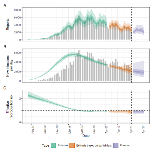

plot(estimates_r0)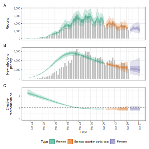

Step 4: Check prior predictive distributions

It is good practice to check if your priors generate reasonable trajectories before seeing data:

# You can visualise prior choices using EpiNow2's distribution objects
prior_r0 <- LogNormal(mean = 2, sd = 0.5, max = 10)
plot(prior_r0)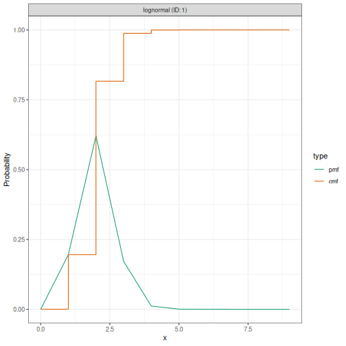

This shows the probability density of your prior. Check if this range is sensible for your application. For example, does it put reasonable mass on plausible $R_0$ values for your pathogen?

Note: Full prior predictive checks (simulating complete epidemic trajectories) require additional Stan code not currently exposed in EpiNow2, but visualising individual prior distributions as shown above is a useful first step.

Step 5: Check model convergence

After modifying priors, always check that the model has converged properly. Poor prior choices can lead to convergence problems.

# Check convergence diagnostics
# Extract the Stan fit object
fit <- estimates_r0$fit

# Check Rhat (should be < 1.01)
summarise_draws(fit, "rhat")
#> # A tibble: 511 × 2
#>    variable   rhat
#>    <chr>     <dbl>
#>  1 params[1] 1.01 
#>  2 params[2] 0.997
#>  3 params[3] 0.988
#>  4 params[4] 1.04 
#>  5 eta[1]    1.00 
#>  6 eta[2]    0.990
#>  7 eta[3]    1.03 
#>  8 eta[4]    1.01 
#>  9 eta[5]    1.06 
#> 10 eta[6]    0.993
#> # ℹ 501 more rows

# Check effective sample size (should be > 400 for reliable inference)
summarise_draws(fit, "ess_bulk", "ess_tail")
#> Warning: The ESS has been capped to avoid unstable estimates.
#> Warning: The ESS has been capped to avoid unstable estimates.
#> Warning: The ESS has been capped to avoid unstable estimates.
#> Warning: The ESS has been capped to avoid unstable estimates.
#> Warning: The ESS has been capped to avoid unstable estimates.
#> Warning: The ESS has been capped to avoid unstable estimates.
#> # A tibble: 511 × 3
#>    variable  ess_bulk ess_tail
#>    <chr>        <dbl>    <dbl>
#>  1 params[1]     72.3     77.5
#>  2 params[2]     97.2     90.1
#>  3 params[3]    146.     119. 
#>  4 params[4]     64.2     36.1
#>  5 eta[1]        87.9     55.3
#>  6 eta[2]        97.0     56.1
#>  7 eta[3]        53.6    102. 
#>  8 eta[4]        79.6     68.1
#>  9 eta[5]        46.7     50.5
#> 10 eta[6]        79.3     60.3
#> # ℹ 501 more rows

# You can also use the summary method which includes these diagnostics
summary(estimates_r0)
#>                         measure                 estimate
#>                          <char>                   <char>
#> 1:       New infections per day       1724 (803 -- 4638)
#> 2:   Expected change in reports        Likely decreasing
#> 3:   Effective reproduction no.       0.88 (0.72 -- 1.1)
#> 4:               Rate of growth -0.032 (-0.082 -- 0.027)
#> 5: Doubling/halving time (days)         -22 (25 -- -8.5)

Key diagnostics to check:

Rhat: Should be < 1.01 for all parameters. Values > 1.01 indicate chains have not converged.
Effective sample size (ESS): Bulk ESS and tail ESS should both be > 400. Low ESS means high autocorrelation and unreliable estimates.
Divergent transitions: Check for warnings about divergences, which indicate problems with the posterior geometry.

If you encounter convergence problems after changing priors, consider:

Making priors less informative (wider)
Checking that prior ranges are sensible (e.g., not excluding plausible parameter values)
Increasing the number of warmup iterations or sampling iterations

Common pitfalls and recommendations

Pitfall 1: Over-informative priors without justification

Problem: Setting very tight priors (small SD) without strong external evidence.

Solution: Use weakly informative priors unless you have literature or prior data supporting tight priors. When in doubt, make priors wider rather than tighter.

Pitfall 2: Ignoring generation time and delays

Problem: Using default gt_opts() and delay_opts(), which assume 1-day generation time and no delays.

Solution: Always specify generation time and delays from literature for your pathogen and data type.

Pitfall 3: Estimating too many uncertain parameters

Problem: Making generation time, delays, and scaling all uncertain in a short time series.

Solution: Prioritize fixed parameters from literature. Only estimate parameters that are truly unknown and have sufficient data (usually >60 days) to identify them.

Pitfall 4: Wrong time scale for length scale

Problem: Setting GP length scale to 1-2 days, expecting very flexible $R_t$ .

Solution: If you want daily flexibility, use a random walk (rt_opts(rw = 1)) rather than GP with very short length scale. GPs with length scale <7 days often struggle.

Pitfall 5: Forgetting the max parameter

Problem: Not setting max on distributions, leading to very long tails and slow computation.

Solution: Always set sensible max values for generation time and delays (e.g., max = 14 or max = 20 for most respiratory diseases).

References and further reading

Mathematical details: See Model definition vignette for full equations and mathematical notation
Gaussian Process details: See Gaussian Process implementation details for GP mathematics
Practical examples: See Examples: estimate_infections() for code examples of different model configurations
Distribution interface: Run ?EpiNow2::Distributions for syntax of specifying distributions

Key papers

For background on renewal equation models:

Cori et al. (2013) on time-varying reproduction numbers: doi:10.1093/aje/kwt133
Riutort-Mayol et al. (2020) on approximate Gaussian processes in Stan: arXiv:2004.11408

Introduction

Set up

Overview of all priors

estimate_infections() priors

estimate_secondary() priors

estimate_truncation() priors

Prior impacts and choice guidance

Reproduction number

Gaussian Process length scale

Gaussian Process magnitude

Random walk for RtR_t (alternative to GP)

Observation model: overdispersion

Observation model: scaling

For estimate_infections():

For estimate_secondary():

For estimate_infections():

For estimate_secondary():

Generation time distribution

Delays (incubation and reporting)

Truncation

Model choice in estimate_infections()

Priors for estimate_secondary()

Delay between primary and secondary

Priors for estimate_truncation()

Truncation distribution parameters

Practical workflow for prior specification

Step 1: Start with defaults

Step 2: Identify candidates for modification

Step 3: Modify one prior at a time

Step 4: Check prior predictive distributions

Step 5: Check model convergence

Common pitfalls and recommendations

Pitfall 1: Over-informative priors without justification

Pitfall 2: Ignoring generation time and delays

Pitfall 3: Estimating too many uncertain parameters

Pitfall 4: Wrong time scale for length scale

Pitfall 5: Forgetting the max parameter

References and further reading

Key papers

Random walk for $R_t$ (alternative to GP)