The scoringutils package provides a collection
of metrics and proper scoring rules that make it simple to score
probabilistic forecasts against observed values. You can find more
information in the paper Evaluating Forecasts with
scoringutils in R as well as the Metrics-Vignette
and the Scoring
forecasts directly Vignette.
The scoringutils package offers convenient automated
forecast evaluation in a data.table format (using the
function score()), but also provides experienced users with
a set of reliable lower-level scoring metrics operating on
vectors/matriced they can build upon in other applications. In addition
it implements a wide range of flexible plots that are able to cover many
use cases.
The goal of this package is to provide a tested and reliable
collection of metrics that can be used for scoring probabilistic
forecasts (forecasts with a full predictive distribution, rather than
point forecasts). It has a much stronger focus on convenience than
e.g. the scoringRules package, which provides a
comprehensive collection of proper scoring rules (also used in
scoringutils). In contrast to other packages,
scoringutils offers functionality to automatically evaluate
forecasts, to visualise scores and to obtain relative scores between
models.
Predictions can be handled in various formats:
scoringutils can handle probabilistic forecasts in either a
sample based or a quantile based format. For more detail on the expected
input formats please see below. True values can be integer, continuous
or binary.
Input formats
Most of the time, the score() function will be able to
do the entire evaluation for you. All you need to do is to pass in a
data.frame with the appropriate columns. Which columns are
required depends on the format the forecasts come in. The forecast
format can either be based on quantiles (see
example_quantile for the expected format), based on
predictive samples (see example_sample_continuous and
example_sample_discrete for the expected format in each
case) or in a binary format. The following table gives an overview
(pairwise comparisons will be explained in more detail below):
| Format | Required columns |
|---|---|
| quantile-based | ‘observed’, ‘predicted’, ‘quantile’ |
| sample-based | ‘observed’, ‘predicted’, ‘sample’ |
| binary | ‘observed’, ‘predicted’ |
| pairwise-comparisons | additionally a column ‘model’ |
Additional columns may be present to indicate a grouping of
forecasts. For example, we could have forecasts made by different models
in various locations at different time points, each for several weeks
into the future. scoringutils automatically tries to
determine the unit of a single forecast, i.e. the combination
of existing columns that are able to uniquely identify a single
forecast. It uses all existing columns for this, which can sometimes
lead to issues. We therefore recommend using the function
set_forecast_unit() to determine the forecast unit
manually. The function simply drops unneeded columns, while making sure
that some necessary, ‘protected columns’ like “predicted” or “observed”
are retained.
colnames(example_quantile)
#>  [1] "location"        "target_end_date" "target_type"     "observed"
#>  [5] "location_name"   "forecast_date"   "quantile_level"  "predicted"
#>  [9] "model"           "horizon"
set_forecast_unit(
  example_quantile,
  c("location", "target_end_date", "target_type", "horizon", "model")
) %>%
  colnames()
#> [1] "observed"        "quantile_level"  "predicted"       "location"
#> [5] "target_end_date" "target_type"     "horizon"         "model"
Constructing a forecast object
The function as_forecast() is be used to construct a
forecast object and check the input data. It determines the forecast
type, creates an object of the appropriate class
(forecast_binary, forecast_quantile or
forecast_sample), and validates the input data. Objects of
class forecast_* have a print method that provides
additional information.
head(example_quantile)
#> Key: <location, target_end_date, target_type>
#>    location target_end_date target_type observed location_name forecast_date
#>      <char>          <Date>      <char>    <num>        <char>        <Date>
#> 1:       DE      2021-01-02       Cases   127300       Germany          <NA>
#> 2:       DE      2021-01-02      Deaths     4534       Germany          <NA>
#> 3:       DE      2021-01-09       Cases   154922       Germany          <NA>
#> 4:       DE      2021-01-09      Deaths     6117       Germany          <NA>
#> 5:       DE      2021-01-16       Cases   110183       Germany          <NA>
#> 6:       DE      2021-01-16      Deaths     5867       Germany          <NA>
#>    quantile_level predicted  model horizon
#>             <num>     <int> <char>   <num>
#> 1:             NA        NA   <NA>      NA
#> 2:             NA        NA   <NA>      NA
#> 3:             NA        NA   <NA>      NA
#> 4:             NA        NA   <NA>      NA
#> 5:             NA        NA   <NA>      NA
#> 6:             NA        NA   <NA>      NA
forecast_quantile <- example_quantile %>%
  set_forecast_unit(
    c("model", "location", "target_end_date", "forecast_date",
      "target_type", "horizon")
  ) %>%
  as_forecast()
#> ℹ Some rows containing NA values may be removed. This is fine if not
#>   unexpected.
forecast_quantile
#> Forecast type: quantile
#> Forecast unit:
#> model, location, target_end_date, forecast_date, target_type, and horizon
#>
#> Key: <location, target_end_date, target_type>
#>        observed quantile_level predicted                model location
#>           <num>          <num>     <int>               <char>   <char>
#>     1:   127300             NA        NA                 <NA>       DE
#>     2:     4534             NA        NA                 <NA>       DE
#>     3:   154922             NA        NA                 <NA>       DE
#>     4:     6117             NA        NA                 <NA>       DE
#>     5:   110183             NA        NA                 <NA>       DE
#>    ---
#> 20541:       78          0.850       352 epiforecasts-EpiNow2       IT
#> 20542:       78          0.900       397 epiforecasts-EpiNow2       IT
#> 20543:       78          0.950       499 epiforecasts-EpiNow2       IT
#> 20544:       78          0.975       611 epiforecasts-EpiNow2       IT
#> 20545:       78          0.990       719 epiforecasts-EpiNow2       IT
#>        target_end_date forecast_date target_type horizon
#>                 <Date>        <Date>      <char>   <num>
#>     1:      2021-01-02          <NA>       Cases      NA
#>     2:      2021-01-02          <NA>      Deaths      NA
#>     3:      2021-01-09          <NA>       Cases      NA
#>     4:      2021-01-09          <NA>      Deaths      NA
#>     5:      2021-01-16          <NA>       Cases      NA
#>    ---
#> 20541:      2021-07-24    2021-07-12      Deaths       2
#> 20542:      2021-07-24    2021-07-12      Deaths       2
#> 20543:      2021-07-24    2021-07-12      Deaths       2
#> 20544:      2021-07-24    2021-07-12      Deaths       2
#> 20545:      2021-07-24    2021-07-12      Deaths       2
If you are unsure what your input data should look like, have a look
at the example_quantile,
example_sample_discrete,
example_sample_continuous and example_binary
data sets provided in the package.
The output of as_forecast() can later be directly used
as input to score(). This is the recommended workflow
(however, score() will run as_forecast()
internally if this hasn’t happened before).
Note that in the above example some columns contain duplicated information with regards to the forecast unit, e.g. “location” and “location_name”, and can be dropped. If we drop essential information, for example, the “target_type” column, we’ll get an error informing us that the forecasts aren’t uniquely identified any more.
example_quantile %>%
  set_forecast_unit(
    c("location", "target_end_date",
      "forecast_date", "model", "horizon")
  ) %>%
  as_forecast()
#> Error: Assertion on 'data' failed: There are instances with more than one forecast for the same target. This can't be right and needs to be resolved. Maybe you need to check the unit of a single forecast and add missing columns? Use the function get_duplicate_forecasts() to identify duplicate rows.
The function get_duplicate_forecasts() may help to
investigate the issue. When filtering for only a single quantile of the
EuroCOVIDhub-ensemble, we can see that there are indeed two forecasts
for every date, location and horizon.
duplicates <- example_quantile %>%
  set_forecast_unit(
    c("location", "target_end_date",
      "forecast_date", "model", "horizon")
  ) %>%
  get_duplicate_forecasts()

duplicates[quantile_level == 0.5 & model == "EuroCOVIDhub-ensemble", ] %>%
  head()
#> Key: <location, target_end_date>
#>    observed quantile_level predicted location target_end_date forecast_date
#>       <num>          <num>     <int>   <char>          <Date>        <Date>
#> 1:   106987            0.5    119258       DE      2021-05-08    2021-05-03
#> 2:     1582            0.5      1568       DE      2021-05-08    2021-05-03
#> 3:    64985            0.5    110716       DE      2021-05-15    2021-05-03
#> 4:    64985            0.5     92649       DE      2021-05-15    2021-05-10
#> 5:     1311            0.5      1521       DE      2021-05-15    2021-05-03
#> 6:     1311            0.5      1422       DE      2021-05-15    2021-05-10
#>                    model horizon
#>                   <char>   <num>
#> 1: EuroCOVIDhub-ensemble       1
#> 2: EuroCOVIDhub-ensemble       1
#> 3: EuroCOVIDhub-ensemble       2
#> 4: EuroCOVIDhub-ensemble       1
#> 5: EuroCOVIDhub-ensemble       2
#> 6: EuroCOVIDhub-ensemble       1
Showing available forecasts
The function get_forecast_counts() may also be helpful
to determine where forecasts are available. Using the by
argument you can specify the level of summary. For example, to see how
many forecasts there are per model and target_type, we can run
get_forecast_counts(forecast_quantile, by = c("model", "target_type"))
#> Key: <model, target_type>
#>                    model target_type count
#>                   <char>      <char> <int>
#> 1: EuroCOVIDhub-baseline       Cases   128
#> 2: EuroCOVIDhub-baseline      Deaths   128
#> 3: EuroCOVIDhub-ensemble       Cases   128
#> 4: EuroCOVIDhub-ensemble      Deaths   128
#> 5:       UMass-MechBayes       Cases     0
#> 6:       UMass-MechBayes      Deaths   128
#> 7:  epiforecasts-EpiNow2       Cases   128
#> 8:  epiforecasts-EpiNow2      Deaths   119
We see that ‘epiforecasts-EpiNow2’ has some missing forecasts for the deaths forecast target and that UMass-MechBayes has no case forecasts.
This information can also be visualised using
plot():
forecast_quantile %>%
  get_forecast_counts(by = c("model", "forecast_date", "target_type")) %>%
  plot_forecast_counts(x = "forecast_date") +
  facet_wrap(~ target_type)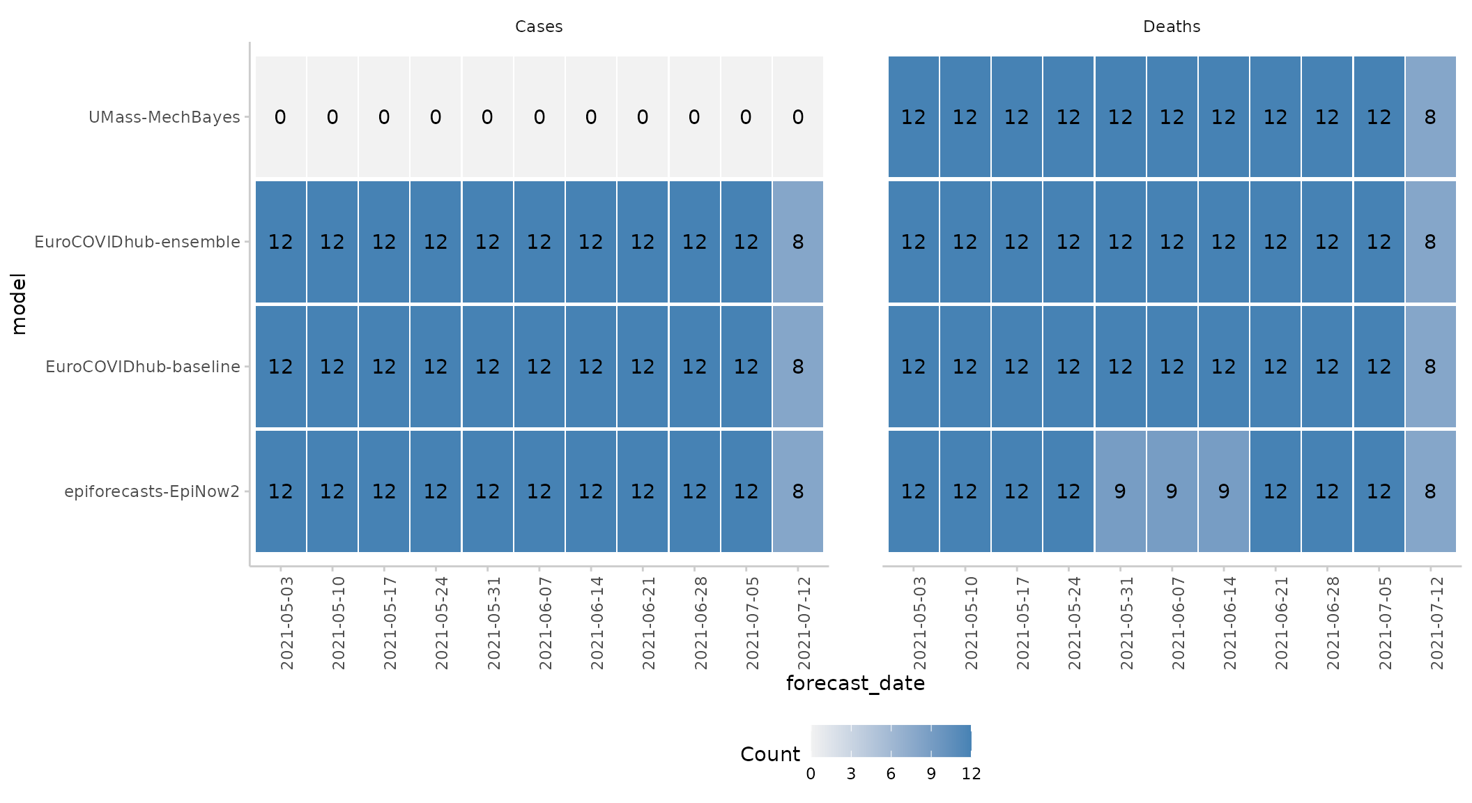
Scoring and summarising forecasts
Forecasts can easily be scored using the score()
function.
For clarity, we suggest setting the forecast unit explicitly and
calling as_forecast() explicitly.
scores <- forecast_quantile %>%
  score()

print(scores, 2)
#>                      model location target_end_date forecast_date target_type
#>                     <char>   <char>          <Date>        <Date>      <char>
#>   1: EuroCOVIDhub-ensemble       DE      2021-05-08    2021-05-03       Cases
#>   2: EuroCOVIDhub-baseline       DE      2021-05-08    2021-05-03       Cases
#>  ---
#> 886:  epiforecasts-EpiNow2       IT      2021-07-24    2021-07-05      Deaths
#> 887:  epiforecasts-EpiNow2       IT      2021-07-24    2021-07-12      Deaths
#>      horizon         wis overprediction underprediction dispersion  bias
#>        <num>       <num>          <num>           <num>      <num> <num>
#>   1:       1  7990.85478    2549.869565               0 5440.98522  0.50
#>   2:       1 16925.04696   15275.826087               0 1649.22087  0.95
#>  ---
#> 886:       3    19.76261       5.478261               0   14.28435  0.50
#> 887:       2    66.16174      40.608696               0   25.55304  0.90
#>      interval_coverage_50 interval_coverage_90 interval_coverage_deviation
#>                    <lgcl>               <lgcl>                       <num>
#>   1:                 TRUE                 TRUE                  0.05181818
#>   2:                FALSE                FALSE                 -0.40272727
#>  ---
#> 886:                 TRUE                 TRUE                  0.05181818
#> 887:                FALSE                 TRUE                 -0.31181818
#>      ae_median
#>          <num>
#>   1:     12271
#>   2:     25620
#>  ---
#> 886:        26
#> 887:       108
The function score() returns unsumarised scores, which
in most cases is not what the user wants. It returns a single score per
forecast (as determined by the forecast unit).
A second function, summarise_scores() takes care of
summarising these scores to the level specified by the user. The
by argument can be used to define the level of summary. By
default, by = model and one score per model is returned.
Through the by argument we can specify what unit of summary
we want. We can also call sumarise_scores() multiple tines,
e.g to round your outputs by specifying e.g. signif() as a
summary function.
scores %>%
  summarise_scores(by = c("model", "target_type")) %>%
  summarise_scores(fun = signif, digits = 2) %>%
kable()| model | wis | overprediction | underprediction | dispersion | bias | interval_coverage_50 | interval_coverage_90 | interval_coverage_deviation | ae_median |
|---|---|---|---|---|---|---|---|---|---|
| EuroCOVIDhub-ensemble | 18000 | 10000.0 | 4200.0 | 3700 | -0.0560 | 0.39 | 0.80 | -0.100 | 24000 |
| EuroCOVIDhub-ensemble | 41 | 7.1 | 4.1 | 30 | 0.0730 | 0.88 | 1.00 | 0.200 | 53 |
| EuroCOVIDhub-baseline | 28000 | 14000.0 | 10000.0 | 4100 | 0.0980 | 0.33 | 0.82 | -0.120 | 38000 |
| EuroCOVIDhub-baseline | 160 | 66.0 | 2.1 | 91 | 0.3400 | 0.66 | 1.00 | 0.120 | 230 |
| epiforecasts-EpiNow2 | 21000 | 12000.0 | 3300.0 | 5700 | -0.0790 | 0.47 | 0.79 | -0.070 | 28000 |
| epiforecasts-EpiNow2 | 67 | 19.0 | 16.0 | 32 | -0.0051 | 0.42 | 0.91 | -0.045 | 100 |
| UMass-MechBayes | 53 | 9.0 | 17.0 | 27 | -0.0220 | 0.46 | 0.88 | -0.025 | 78 |
Scoring point forecasts
Point forecasts can be scored in a separate format.
suppressMessages(score(as_forecast(example_point))) %>%
  summarise_scores(by = "model", na.rm = TRUE)
#>                    model    ae_point     se_point       ape
#>                   <char>       <num>        <num>     <num>
#> 1: EuroCOVIDhub-ensemble 12077.10156 1.945118e+09 0.2996696
#> 2: EuroCOVIDhub-baseline 19353.42969 2.883446e+09 0.7383936
#> 3:  epiforecasts-EpiNow2 14521.10526 2.680928e+09 0.3715552
#> 4:       UMass-MechBayes    78.47656 1.170976e+04 0.2823206
Adding empirical coverage
For quantile-based forecasts we are often interested in specific
coverage-levels, for example, what percentage of true values fell
between all 50% or the 90% prediction intervals. We can add this
information using the function get_coverage(). This
function also requires a by argument which defines the
level of grouping for which the percentage of true values covered by
certain prediction intervals is computed.
score(as_forecast(example_quantile)) %>%
  summarise_scores(by = c("model", "target_type")) %>%
  summarise_scores(fun = signif, digits = 2)
#> ℹ Some rows containing NA values may be removed. This is fine if not
#>   unexpected.
#>                    model   wis overprediction underprediction dispersion
#>                   <char> <num>          <num>           <num>      <num>
#> 1: EuroCOVIDhub-ensemble 18000        10000.0          4200.0       3700
#> 2: EuroCOVIDhub-ensemble    41            7.1             4.1         30
#> 3: EuroCOVIDhub-baseline 28000        14000.0         10000.0       4100
#> 4: EuroCOVIDhub-baseline   160           66.0             2.1         91
#> 5:  epiforecasts-EpiNow2 21000        12000.0          3300.0       5700
#> 6:  epiforecasts-EpiNow2    67           19.0            16.0         32
#> 7:       UMass-MechBayes    53            9.0            17.0         27
#>       bias interval_coverage_50 interval_coverage_90
#>      <num>                <num>                <num>
#> 1: -0.0560                 0.39                 0.80
#> 2:  0.0730                 0.88                 1.00
#> 3:  0.0980                 0.33                 0.82
#> 4:  0.3400                 0.66                 1.00
#> 5: -0.0790                 0.47                 0.79
#> 6: -0.0051                 0.42                 0.91
#> 7: -0.0220                 0.46                 0.88
#>    interval_coverage_deviation ae_median
#>                          <num>     <num>
#> 1:                      -0.100     24000
#> 2:                       0.200        53
#> 3:                      -0.120     38000
#> 4:                       0.120       230
#> 5:                      -0.070     28000
#> 6:                      -0.045       100
#> 7:                      -0.025        78
Adding relative scores
In order to better compare models against each other we can use
relative scores which are computed based on pairwise comparisons (see
details below). Relative scores can be added to the evaluation using the
function summarise_scores(). This requires a column called
‘model’ to be present. Pairwise comparisons are computed according to
the grouping specified in by: essentially, the data.frame
with all scores gets split into different data.frames according to the
values specified in by and relative scores are computed for
every individual group separately. The baseline argument
allows us to specify a baseline that can be used to scale relative
scores (all scores are divided by the baseline relative score). For
example, to obtain relative scores separately for different forecast
targets, we can run
score(as_forecast(example_quantile)) %>%
  add_relative_skill(
    by = c("model", "target_type"),
    baseline = "EuroCOVIDhub-ensemble"
  ) %>%
  summarise_scores(by = c("model", "target_type"))
#> ℹ Some rows containing NA values may be removed. This is fine if not
#>   unexpected.
#> Key: <model, target_type>
#>                    model target_type         wis overprediction underprediction
#>                   <char>      <char>       <num>          <num>           <num>
#> 1: EuroCOVIDhub-baseline       Cases 28483.57465   14096.100883    10284.972826
#> 2: EuroCOVIDhub-baseline      Deaths   159.40387      65.899117        2.098505
#> 3: EuroCOVIDhub-ensemble       Cases 17943.82383   10043.121943     4237.177310
#> 4: EuroCOVIDhub-ensemble      Deaths    41.42249       7.138247        4.103261
#> 5:       UMass-MechBayes      Deaths    52.65195       8.978601       16.800951
#> 6:  epiforecasts-EpiNow2       Cases 20831.55662   11906.823030     3260.355639
#> 7:  epiforecasts-EpiNow2      Deaths    66.64282      18.892583       15.893314
#>    dispersion        bias interval_coverage_50 interval_coverage_90
#>         <num>       <num>                <num>                <num>
#> 1: 4102.50094  0.09796875            0.3281250            0.8203125
#> 2:   91.40625  0.33906250            0.6640625            1.0000000
#> 3: 3663.52458 -0.05640625            0.3906250            0.8046875
#> 4:   30.18099  0.07265625            0.8750000            1.0000000
#> 5:   26.87239 -0.02234375            0.4609375            0.8750000
#> 6: 5664.37795 -0.07890625            0.4687500            0.7890625
#> 7:   31.85692 -0.00512605            0.4201681            0.9075630
#>    interval_coverage_deviation   ae_median wis_relative_skill
#>                          <num>       <num>              <num>
#> 1:                 -0.11721591 38473.60156          1.2947445
#> 2:                  0.12142045   233.25781          2.2958723
#> 3:                 -0.10230114 24101.07031          0.8156514
#> 4:                  0.20380682    53.13281          0.5966310
#> 5:                 -0.02488636    78.47656          0.7475873
#> 6:                 -0.06963068 27923.81250          0.9469157
#> 7:                 -0.04520244   104.74790          0.9765276
#>    wis_scaled_relative_skill
#>                        <num>
#> 1:                  1.587375
#> 2:                  3.848060
#> 3:                  1.000000
#> 4:                  1.000000
#> 5:                  1.253014
#> 6:                  1.160932
#> 7:                  1.636736
Visualising scores
Score heatmap
We can also summarise one particular metric across different categories using a simple heatmap:
score(as_forecast(example_sample_continuous)) %>%
  summarise_scores(by = c("model", "location", "target_type")) %>%
  plot_heatmap(x = "location", metric = "bias") +
  facet_wrap(~ target_type)
#> ℹ Some rows containing NA values may be removed. This is fine if not
#>   unexpected.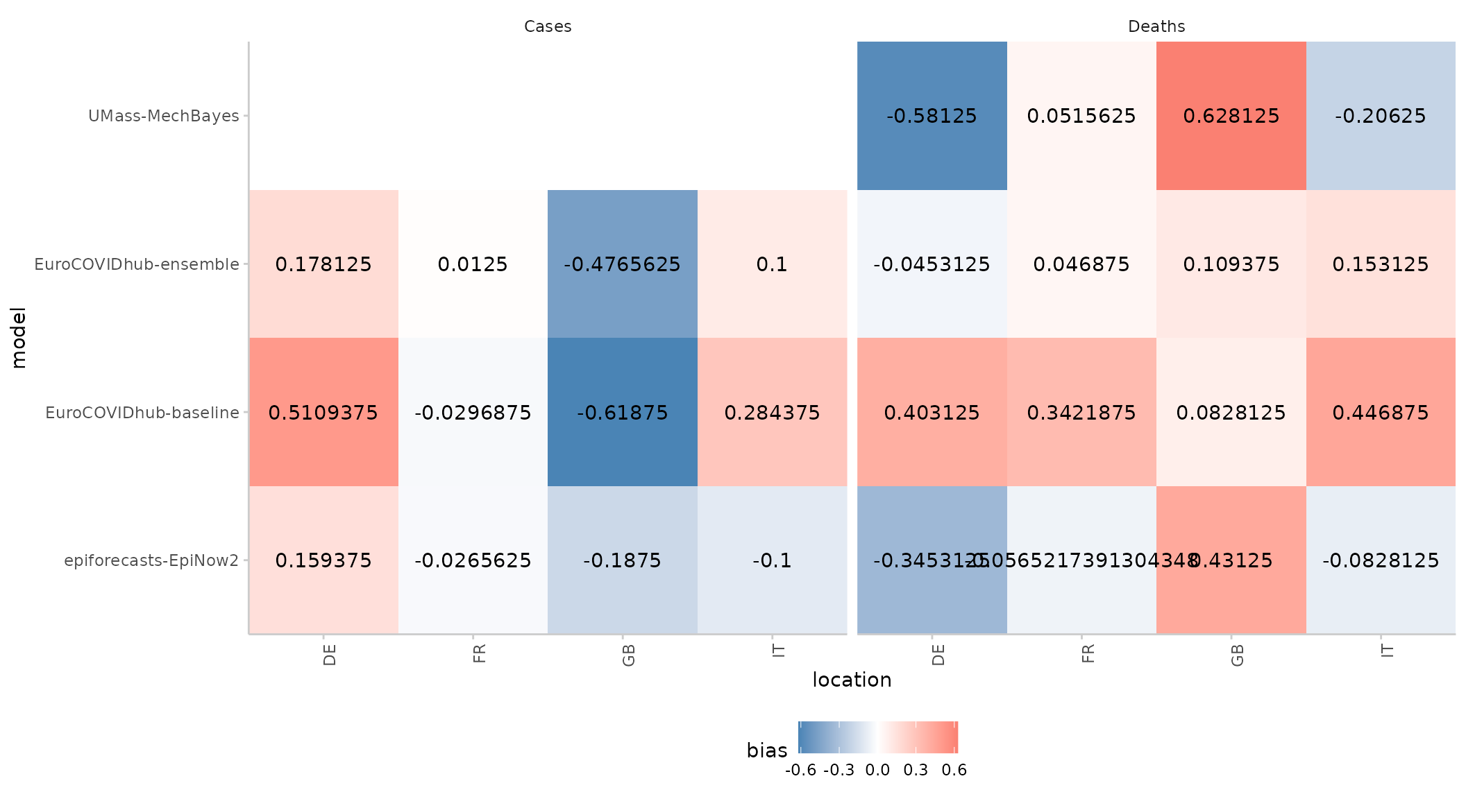
Weighted interval score components
The weighted interval score can be split up into three components: Over-prediction, under-prediction and dispersion. These can be visualised separately in the following way:
score(as_forecast(example_quantile)) %>%
  summarise_scores(by = c("target_type", "model")) %>%
  plot_wis() +
  facet_wrap(~ target_type, scales = "free")
#> ℹ Some rows containing NA values may be removed. This is fine if not
#>   unexpected.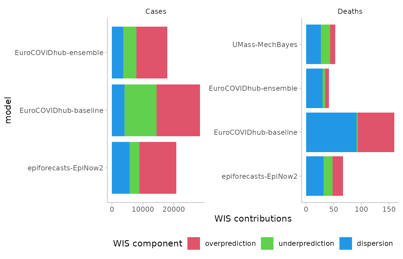
Calibration
Calibration is a measure statistical consistency between the forecasts and observed values. The most common way of assessing calibration (more precisely: probabilistic calibration) are PIT histograms. The probability integral transform (PIT) is equal to the cumulative distribution function of a forecast evaluated at the observed value. Ideally, pit values should be uniformly distributed after the transformation.
We can compute pit values as such:
example_sample_continuous %>%
  as_forecast() %>%
  get_pit(by = "model")
#> ℹ Some rows containing NA values may be removed. This is fine if not
#>   unexpected.
#>                      model pit_value
#>                     <char>     <num>
#>   1: EuroCOVIDhub-baseline     0.025
#>   2: EuroCOVIDhub-baseline     0.525
#>   3: EuroCOVIDhub-baseline     0.000
#>   4: EuroCOVIDhub-baseline     0.000
#>   5: EuroCOVIDhub-baseline     0.200
#>  ---
#> 883:       UMass-MechBayes     0.950
#> 884:       UMass-MechBayes     0.500
#> 885:       UMass-MechBayes     0.100
#> 886:       UMass-MechBayes     0.450
#> 887:       UMass-MechBayes     0.100
And visualise the results as such:
example_sample_continuous %>%
  as_forecast() %>%
  get_pit(by = c("model", "target_type")) %>%
  plot_pit() +
  facet_grid(model ~ target_type)
#> ℹ Some rows containing NA values may be removed. This is fine if not
#>   unexpected.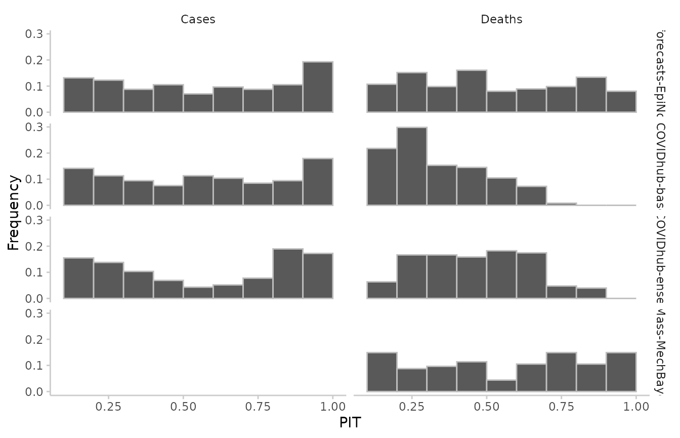
Similarly for quantile-based forecasts:
example_quantile[quantile_level %in% seq(0.1, 0.9, 0.1), ] %>%
  as_forecast() %>%
  get_pit(by = c("model", "target_type")) %>%
  plot_pit() +
  facet_grid(model ~ target_type)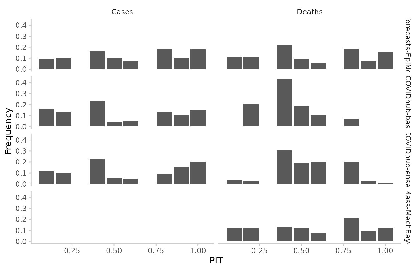
Pairwise comparisons
Relative scores for different models can be computed using pairwise comparisons, a sort of pairwise tournament where all combinations of two models are compared against each other based on the overlapping set of available forecasts common to both models. Internally, a ratio of the mean scores of both models is computed. The relative score of a model is then the geometric mean of all mean score ratios which involve that model. When a baseline is provided, then that baseline is excluded from the relative scores for individual models (which therefore differ slightly from relative scores without a baseline) and all relative scores are scaled by (i.e. divided by) the relative score of the baseline model.
In scoringutils, pairwise comparisons can be made in two
ways: Through the standalone function
get_pairwise_comparisons() or from within
summarise_scores() which simply adds relative scores to an
existing set of scores.
forecast_quantile %>%
  score() %>%
  get_pairwise_comparisons(by = "model", baseline = "EuroCOVIDhub-baseline")
#>                     model       compare_against mean_scores_ratio         pval
#>                    <char>                <char>             <num>        <num>
#>  1: EuroCOVIDhub-baseline  epiforecasts-EpiNow2         1.3703452 9.164893e-18
#>  2: EuroCOVIDhub-baseline       UMass-MechBayes         3.0275019 2.627464e-20
#>  3: EuroCOVIDhub-baseline EuroCOVIDhub-ensemble         1.5925819 2.608666e-32
#>  4: EuroCOVIDhub-baseline EuroCOVIDhub-baseline         1.0000000 1.000000e+00
#>  5: EuroCOVIDhub-ensemble EuroCOVIDhub-baseline         0.6279112 2.608666e-32
#>  6: EuroCOVIDhub-ensemble       UMass-MechBayes         0.7867229 1.244731e-04
#>  7: EuroCOVIDhub-ensemble  epiforecasts-EpiNow2         0.8606607 1.881520e-02
#>  8: EuroCOVIDhub-ensemble EuroCOVIDhub-ensemble         1.0000000 1.000000e+00
#>  9:       UMass-MechBayes EuroCOVIDhub-ensemble         1.2710955 1.244731e-04
#> 10:       UMass-MechBayes  epiforecasts-EpiNow2         0.7439673 7.253878e-03
#> 11:       UMass-MechBayes EuroCOVIDhub-baseline         0.3303053 2.627464e-20
#> 12:       UMass-MechBayes       UMass-MechBayes         1.0000000 1.000000e+00
#> 13:  epiforecasts-EpiNow2       UMass-MechBayes         1.3441452 7.253878e-03
#> 14:  epiforecasts-EpiNow2 EuroCOVIDhub-ensemble         1.1618981 1.881520e-02
#> 15:  epiforecasts-EpiNow2 EuroCOVIDhub-baseline         0.7297431 9.164893e-18
#> 16:  epiforecasts-EpiNow2  epiforecasts-EpiNow2         1.0000000 1.000000e+00
#>         adj_pval wis_relative_skill wis_scaled_relative_skill
#>            <num>              <num>                     <num>
#>  1: 3.665957e-17          1.6032604                 1.0000000
#>  2: 1.313732e-19          1.6032604                 1.0000000
#>  3: 1.565200e-31          1.6032604                 1.0000000
#>  4: 1.000000e+00          1.6032604                 1.0000000
#>  5: 1.565200e-31          0.8074916                 0.5036559
#>  6: 3.734192e-04          0.8074916                 0.5036559
#>  7: 1.881520e-02          0.8074916                 0.5036559
#>  8: 1.000000e+00          0.8074916                 0.5036559
#>  9: 3.734192e-04          0.7475873                 0.4662919
#> 10: 1.450776e-02          0.7475873                 0.4662919
#> 11: 1.313732e-19          0.7475873                 0.4662919
#> 12: 1.000000e+00          0.7475873                 0.4662919
#> 13: 1.450776e-02          1.0332277                 0.6444541
#> 14: 1.881520e-02          1.0332277                 0.6444541
#> 15: 3.665957e-17          1.0332277                 0.6444541
#> 16: 1.000000e+00          1.0332277                 0.6444541
forecast_quantile %>%
  score() %>%
  summarise_scores(by = "model") %>%
  add_relative_skill(baseline = "EuroCOVIDhub-baseline")
#> Warning: ! `by` is set to 'model', which is also the unit of a single forecast. This
#>   doesn't look right.
#> ℹ All relative skill scores will be equal to 1.
#> Key: <model>
#>                    model         wis overprediction underprediction dispersion
#>                   <char>       <num>          <num>           <num>      <num>
#> 1: EuroCOVIDhub-baseline 14321.48926    7081.000000      5143.53567 2096.95360
#> 2: EuroCOVIDhub-ensemble  8992.62316    5025.130095      2120.64029 1846.85278
#> 3:       UMass-MechBayes    52.65195       8.978601        16.80095   26.87239
#> 4:  epiforecasts-EpiNow2 10827.40786    6179.439535      1697.23411 2950.73422
#>           bias interval_coverage_50 interval_coverage_90
#>          <num>                <num>                <num>
#> 1:  0.21851562            0.4960938            0.9101562
#> 2:  0.00812500            0.6328125            0.9023438
#> 3: -0.02234375            0.4609375            0.8750000
#> 4: -0.04336032            0.4453441            0.8461538
#>    interval_coverage_deviation   ae_median wis_relative_skill
#>                          <num>       <num>              <num>
#> 1:                 0.002102273 19353.42969                  1
#> 2:                 0.050752841 12077.10156                  1
#> 3:                -0.024886364    78.47656                  1
#> 4:                -0.057861612 14521.10526                  1
#>    wis_scaled_relative_skill
#>                        <num>
#> 1:                         1
#> 2:                         1
#> 3:                         1
#> 4:                         1
If using the get_pairwise_comparisons() function, we can
also visualise pairwise comparisons by showing the mean score ratios
between models. By default, smaller values are better and the model we
care about is showing on the y axis on the left, while the model against
it is compared is shown on the x-axis on the bottom. In the example
above, the EuroCOVIDhub-ensemble performs best (it only has values
smaller 1), while the EuroCOVIDhub-baseline performs worst (and only has
values larger than 1). For cases, the UMass-MechBayes model is of course
excluded as there are no case forecasts available and therefore the set
of overlapping forecasts is empty.
forecast_quantile %>%
  score() %>%
  get_pairwise_comparisons(by = c("model", "target_type")) %>%
  plot_pairwise_comparisons() +
  facet_wrap(~ target_type)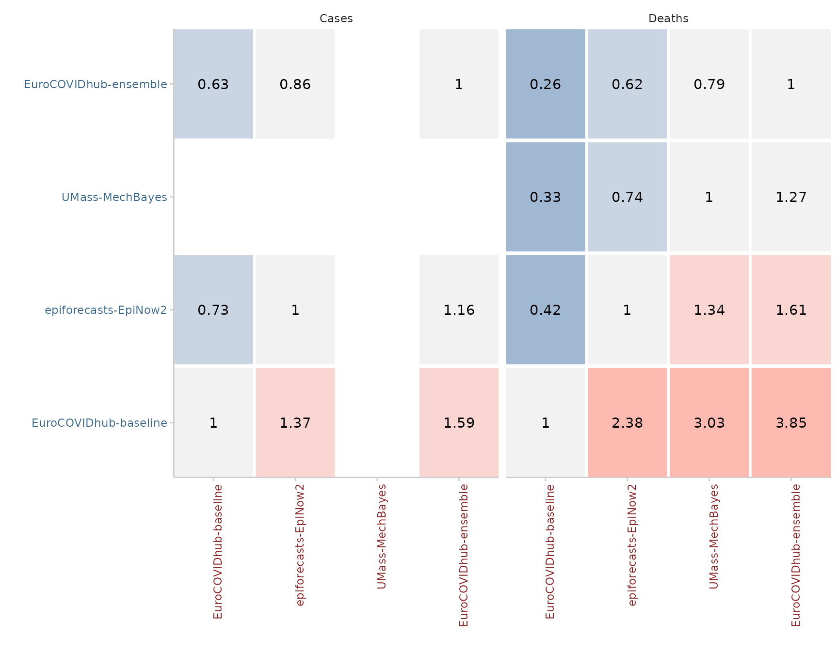
Additional analyses and visualisations
Correlation between scores
It may sometimes be interesting to see how different scores correlate
with each other. We can examine this using the function
correlation(). When dealing with quantile-based forecasts,
it is important to call summarise_scorees() before
get_correlations() to summarise over quantiles before
computing correlations.
forecast_quantile %>%
  score() %>%
  summarise_scores() %>%
  get_correlations()
#>          wis overprediction underprediction  dispersion       bias
#>        <num>          <num>           <num>       <num>      <num>
#> 1: 1.0000000      0.9917884       0.8821058  0.86564717 0.61587946
#> 2: 0.9917884      1.0000000       0.8158534  0.91900505 0.51068021
#> 3: 0.8821058      0.8158534       1.0000000  0.52982259 0.91280769
#> 4: 0.8656472      0.9190050       0.5298226  1.00000000 0.14860643
#> 5: 0.6158795      0.5106802       0.9128077  0.14860643 1.00000000
#> 6: 0.1565567      0.1740382       0.1630289  0.04407105 0.06639491
#> 7: 0.2818348      0.1968480       0.6141229 -0.17841559 0.74137210
#> 8: 0.1364221      0.1123720       0.2954741 -0.12711127 0.30908292
#> 9: 0.9999780      0.9909177       0.8851559  0.86247754 0.62106954
#>    interval_coverage_50 interval_coverage_90 interval_coverage_deviation
#>                   <num>                <num>                       <num>
#> 1:           0.15655670            0.2818348                   0.1364221
#> 2:           0.17403818            0.1968480                   0.1123720
#> 3:           0.16302890            0.6141229                   0.2954741
#> 4:           0.04407105           -0.1784156                  -0.1271113
#> 5:           0.06639491            0.7413721                   0.3090829
#> 6:           1.00000000            0.6417542                   0.9466440
#> 7:           0.64175425            1.0000000                   0.8451292
#> 8:           0.94664396            0.8451292                   1.0000000
#> 9:           0.15565388            0.2861731                   0.1376834
#>    ae_median                      metric
#>        <num>                      <char>
#> 1: 0.9999780                         wis
#> 2: 0.9909177              overprediction
#> 3: 0.8851559             underprediction
#> 4: 0.8624775                  dispersion
#> 5: 0.6210695                        bias
#> 6: 0.1556539        interval_coverage_50
#> 7: 0.2861731        interval_coverage_90
#> 8: 0.1376834 interval_coverage_deviation
#> 9: 1.0000000                   ae_median
Visualising correlations:
forecast_quantile %>%
  score() %>%
  summarise_scores() %>%
  get_correlations(digits = 2) %>%
  plot_correlations()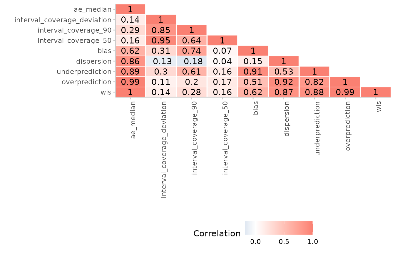
Converting to quantile-based forecasts
Different metrics are available for different forecasting formats. In some cases, you may for example have forecasts in a sample-based format, but wish to make use of some of the functionality only available to quantile-based forecasts. For example, you may want to use the decomposition of the weighted interval score, or may like to compute interval coverage values.
You can convert your sample-based forecasts into a quantile-based
format using the function sample_to_quantile(). There is,
however, one caveat: Quantiles will be calculated based on the
predictive samples, which may introduce a bias if the number of
available samples is small.
example_sample_discrete %>%
  as_forecast() %>%
  sample_to_quantile(
    quantile_level = c(0.01, 0.025, seq(0.05, 0.95, 0.05), 0.975, 0.99)
  ) %>%
  as_forecast() %>%
  score()
#> ℹ Some rows containing NA values may be removed. This is fine if not
#>   unexpected.
#> ℹ Some rows containing NA values may be removed. This is fine if not
#>   unexpected.
#> ℹ Some rows containing NA values may be removed. This is fine if not
#>   unexpected.
#>      location location_name target_end_date target_type forecast_date
#>        <char>        <char>          <Date>      <char>        <Date>
#>   1:       DE       Germany      2021-05-08       Cases    2021-05-03
#>   2:       DE       Germany      2021-05-08       Cases    2021-05-03
#>   3:       DE       Germany      2021-05-08       Cases    2021-05-03
#>   4:       DE       Germany      2021-05-08      Deaths    2021-05-03
#>   5:       DE       Germany      2021-05-08      Deaths    2021-05-03
#>  ---
#> 883:       IT         Italy      2021-07-24      Deaths    2021-07-12
#> 884:       IT         Italy      2021-07-24      Deaths    2021-07-05
#> 885:       IT         Italy      2021-07-24      Deaths    2021-07-12
#> 886:       IT         Italy      2021-07-24      Deaths    2021-07-05
#> 887:       IT         Italy      2021-07-24      Deaths    2021-07-12
#>                      model horizon         wis overprediction underprediction
#>                     <char>   <num>       <num>          <num>           <num>
#>   1: EuroCOVIDhub-ensemble       1  6671.68207   2.110043e+03        0.000000
#>   2: EuroCOVIDhub-baseline       1 18441.13061   1.446498e+04        0.000000
#>   3:  epiforecasts-EpiNow2       1 22042.77309   1.548071e+04        0.000000
#>   4: EuroCOVIDhub-ensemble       1    59.46028   9.682609e+00        0.000000
#>   5: EuroCOVIDhub-baseline       1    75.93215   0.000000e+00        1.195652
#>  ---
#> 883: EuroCOVIDhub-baseline       2    60.71862   1.323913e+01        0.000000
#> 884:       UMass-MechBayes       3     5.79650   3.695652e-01        0.000000
#> 885:       UMass-MechBayes       2    26.18112   1.891304e+01        0.000000
#> 886:  epiforecasts-EpiNow2       3    25.13032   3.478261e-01        0.000000
#> 887:  epiforecasts-EpiNow2       2    44.07931   2.410435e+01        0.000000
#>       dispersion  bias interval_coverage_50 interval_coverage_90
#>            <num> <num>               <lgcl>               <lgcl>
#>   1: 4561.638591  0.60                FALSE                 TRUE
#>   2: 3976.145828  0.98                FALSE                FALSE
#>   3: 6562.060048  0.90                FALSE                 TRUE
#>   4:   49.777674  0.30                 TRUE                 TRUE
#>   5:   74.736502 -0.10                 TRUE                 TRUE
#>  ---
#> 883:   47.479491  0.50                 TRUE                 TRUE
#> 884:    5.426935  0.20                 TRUE                 TRUE
#> 885:    7.268076  0.90                FALSE                 TRUE
#> 886:   24.782489  0.10                 TRUE                 TRUE
#> 887:   19.974959  0.70                FALSE                 TRUE
#>      interval_coverage_deviation ae_median
#>                            <num>     <num>
#>   1:                 -0.03909091    9414.0
#>   2:                 -0.49363636   29379.0
#>   3:                 -0.31181818   36513.0
#>   4:                  0.23363636      77.0
#>   5:                  0.41545455      27.5
#>  ---
#> 883:                  0.05181818      58.5
#> 884:                  0.32454545       5.0
#> 885:                 -0.31181818      42.5
#> 886:                  0.41545455       8.0
#> 887:                 -0.13000000      73.5