Fitting delay distributions with estimate

Introduction

Epidemiological delay distributions are subject to double interval censoring: both the primary event (e.g. infection) and the secondary event (e.g. symptom onset) are observed within discrete time windows rather than at exact times^[1,2]. If ignored, this censoring biases parameter estimates. Right truncation introduces further bias because recent observations are systematically missing due to reporting delays.

estimate_dist() fits delay distributions from linelist data while accounting for both of these biases. Event times are typically recorded at daily resolution, but the date-based interface supports arbitrary censoring window widths. The function uses a Stan model that vendors likelihood functions from the primarycensored package. If you use estimate_dist(), please cite primarycensored in addition to EpiNow2.

Common use cases include estimating the incubation period (infection to symptom onset), the reporting delay (symptom onset to case report), or the serial interval (symptom onset in infector-infectee pairs). Generation time estimation (infection to infection) typically requires known infection times for both infector and infectee, which generally calls for more complex models.

For more flexible delay distribution modelling, epidist supports time-varying delays, partial pooling across delays, regression on covariates, and a range of other models. primarycensored operates at a lower level, working directly with numeric delays and censoring windows. It supports fitting delay distributions both with and without a Stan dependency and is also useful for creating double interval censoring and truncation adjusted probability mass functions for use in other models. primarycensored also supports vendoring its Stan functions into custom models, which is useful for adapting the delay estimation approach to support more complex settings such as additional observation biases, mixture models, or joint estimation with other processes.

Set up

library(EpiNow2) # nolint: unused_import_linter.
library(primarycensored)
library(ggplot2)
options(mc.cores = 2)

Simulating censored delay data

We simulate 200 individual delay observations from a lognormal distribution with known parameters. Each observation has its own primary and secondary censoring window width (1 or 2 days) and its own observation time (8 to 15 days after the primary event), reflecting the kind of variation present in real data.

set.seed(42)
n <- 200

true_meanlog <- 1.5
true_sdlog <- 0.75

pwindows <- sample.int(2, n, replace = TRUE)
swindows <- sample.int(2, n, replace = TRUE)
obs_times <- sample(8:15, n, replace = TRUE)

delays <- mapply(
  function(pw, sw, D) {
    rprimarycensored(
      1, rlnorm,
      meanlog = true_meanlog, sdlog = true_sdlog,
      pwindow = pw, swindow = sw, D = D
    )
  },
  pwindows, swindows, obs_times
)

pdate_lwr <- as.Date("2023-01-01") +
  sample(0:13, n, replace = TRUE)

linelist <- data.frame(
  pdate_lwr = pdate_lwr,
  pdate_upr = pdate_lwr + pwindows,
  sdate_lwr = pdate_lwr + delays,
  sdate_upr = pdate_lwr + delays + swindows,
  obs_date = pdate_lwr + obs_times
)

# Observations where the secondary event window extends
# past the observation date are not yet fully observed and
# would not appear in a real linelist.
linelist <- linelist[linelist$obs_date >= linelist$sdate_upr, ]

head(linelist)
#>    pdate_lwr  pdate_upr  sdate_lwr  sdate_upr   obs_date
#> 1 2023-01-06 2023-01-07 2023-01-14 2023-01-16 2023-01-21
#> 2 2023-01-14 2023-01-15 2023-01-18 2023-01-20 2023-01-25
#> 3 2023-01-01 2023-01-02 2023-01-11 2023-01-12 2023-01-16
#> 4 2023-01-06 2023-01-07 2023-01-10 2023-01-12 2023-01-18
#> 5 2023-01-06 2023-01-08 2023-01-09 2023-01-10 2023-01-21
#> 6 2023-01-14 2023-01-16 2023-01-17 2023-01-18 2023-01-27

observed_delays <- as.numeric(
  linelist$sdate_lwr - linelist$pdate_lwr
)

ggplot(data.frame(delay = observed_delays), aes(x = delay)) +
  geom_histogram(
    aes(y = after_stat(density)),
    binwidth = 1, fill = "#4292C6", colour = "white"
  ) +
  stat_function(
    fun = dlnorm,
    args = list(
      meanlog = true_meanlog, sdlog = true_sdlog
    ),
    linewidth = 1
  ) +
  labs(
    x = "Delay (days)",
    y = "Density",
    title = "Observed delays vs true distribution"
  ) +
  theme_minimal()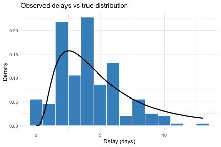

plot of chunk plot-delays

The histogram shows the observed delay lower bounds (i.e. sdate_lwr - pdate_lwr) from the filtered linelist. The solid line shows the true underlying lognormal density. The gap between the two illustrates the bias introduced by censoring and truncation, which estimate_dist() corrects for.

The data frame has five columns:

pdate_lwr: lower bound of the primary event date (e.g. date of infection).
pdate_upr: upper bound of the primary event date.
sdate_lwr: lower bound of the secondary event date (e.g. date of symptom onset).
sdate_upr: upper bound of the secondary event date.
obs_date: the date at which the data were extracted, determining the right truncation point for each observation.

Upper bounds for the primary and secondary event windows default to one day after the lower bounds (daily censoring) if not provided.

Note that the simulation above constructs dates from numeric delays using a dummy origin date. If you have numeric delays without dates, you can do the same thing: set pdate_lwr to an arbitrary origin (e.g. as.Date("2020-01-01")) and derive the other columns by adding the appropriate intervals.

For obs_date, use the date the data were sent to you, or the date data collection stopped. If neither is available, estimate_dist() defaults to max(sdate_upr), which is a reasonable fallback for most situations.

Setting priors

By default, estimate_dist() uses Normal(1, 1) for meanlog and Normal(0.5, 0.5) for sdlog. These are fairly wide and may not reflect domain knowledge. We recommend setting priors based on what you know about the delay.

For meanlog, the prior should reflect the expected median delay on the log scale, since exp(meanlog) is the median of a lognormal (the mean is exp(meanlog + sdlog^2 / 2)). If you expect a delay with a median around 3–7 days, log(5) ≈ 1.6 is a reasonable centre. A standard deviation of 0.5 on the log scale corresponds to roughly a factor of 1.6 uncertainty (since exp(0.5) ≈ 1.6), so the prior covers median delays from about 5/1.6 ≈ 3 to 5 * 1.6 ≈ 8 days within one standard deviation.

For sdlog, it helps to think in terms of the coefficient of variation (CV). For a lognormal distribution, CV = sqrt(exp(sdlog²) - 1) depends only on sdlog. A sdlog of 0.5 gives CV ≈ 0.53 (the standard deviation is about half the mean), while sdlog = 1.0 gives CV ≈ 1.3 (very dispersed). Here we centre on 0.5 because we expect moderate variability in this delay, with a fairly tight prior (sd = 0.25) to rule out very large values.

We define the prior as a dist_spec and use plot() to check that the implied delay distributions are plausible before fitting.

prior_dist <- LogNormal(
  meanlog = Normal(1.6, 0.5),
  sdlog = Normal(0.5, 0.25),
  max = 20
)

plot(prior_dist, samples = 50, cumulative = FALSE)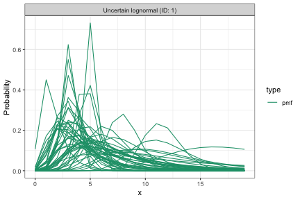

plot of chunk prior-predictive

Each line is a delay distribution drawn from the priors. The range should cover plausible delays for the application without placing substantial weight on unrealistic values.

Fitting the model

We pass the linelist to estimate_dist(), extracting the priors from our dist_spec. Internally the function converts dates to numeric intervals, then aggregates identical delay-censoring-truncation combinations and counts their occurrences. This reduces the number of likelihood evaluations, which speeds up fitting when many observations share the same structure.

result <- estimate_dist(
  linelist,
  dist = "lognormal",
  priors = get_parameters(prior_dist)
)

The result object is an estimate_dist object that inherits from epinowfit. Printing it shows a posterior summary of the fitted parameters.

result
#> Delay distribution: lognormal (max: 14)
#> Observations: 198 (129 unique strata)
#> Primary event: uniform 
#> Max delay: 14 | Max obs time: 15
#> 
#> Parameter estimates:
#>    variable    median      mean         sd  lower_90 lower_50  lower_20
#>      <char>     <num>     <num>      <num>     <num>    <num>     <num>
#> 1:  meanlog 1.4001531 1.4068572 0.09398806 1.2655999 1.343393 1.3759575
#> 2:    sdlog 0.7813516 0.7894131 0.07509719 0.6804412 0.733925 0.7642848
#>     upper_20  upper_50  upper_90
#>        <num>     <num>     <num>
#> 1: 1.4214566 1.4611444 1.5759207
#> 2: 0.8008999 0.8365392 0.9237593

For convergence diagnostics, the underlying Stan fit is accessible via result$fit.

rstan::summary(result$fit)$summary
#>                         mean     se_mean         sd         2.5%         25%
#> params[1]          1.4068572 0.003617471 0.09398806    1.2426296    1.343393
#> params[2]          0.7894131 0.002818455 0.07509719    0.6621815    0.733925
#> delay_params[1]    1.4068572 0.003617471 0.09398806    1.2426296    1.343393
#> delay_params[2]    0.7894131 0.002818455 0.07509719    0.6621815    0.733925
#> lp__            -374.9899611 0.035684411 0.98070943 -377.5335854 -375.388382
#>                          50%          75%        97.5%    n_eff     Rhat
#> params[1]          1.4001531    1.4611444    1.6166435 675.0489 1.003295
#> params[2]          0.7813516    0.8365392    0.9616258 709.9457 1.004643
#> delay_params[1]    1.4001531    1.4611444    1.6166435 675.0489 1.003295
#> delay_params[2]    0.7813516    0.8365392    0.9616258 709.9457 1.004643
#> lp__            -374.6670125 -374.2767613 -374.0051957 755.3072 1.000937

We can extract the fitted distribution as a dist_spec object using get_parameters(). This is useful for passing the result directly to other EpiNow2 functions such as estimate_infections() via delay_opts().

params <- get_parameters(result)
params$delay
#> - lognormal distribution (max: 14):
#>   meanlog:
#>     - normal distribution:
#>       mean:
#>         1.4
#>       sd:
#>         0.094
#>   sdlog:
#>     - normal distribution:
#>       mean:
#>         0.79
#>       sd:
#>         0.075

Checking parameter recovery

We can check how well the model recovers the true parameters by comparing the fitted posterior to the true distribution.

posterior <- extract_samples(
  result$fit, pars = "delay_params"
)
post_meanlog <- posterior$delay_params[, 1]
post_sdlog <- posterior$delay_params[, 2]

param_df <- data.frame(
  value = c(post_meanlog, post_sdlog),
  parameter = rep(
    c("meanlog", "sdlog"),
    each = length(post_meanlog)
  )
)

true_df <- data.frame(
  parameter = c("meanlog", "sdlog"),
  value = c(true_meanlog, true_sdlog)
)

ggplot(param_df, aes(x = value)) +
  geom_density(fill = "#4292C6", alpha = 0.3) +
  geom_vline(
    data = true_df, aes(xintercept = value),
    linetype = "dashed", linewidth = 1
  ) +
  facet_wrap(~parameter, scales = "free") +
  labs(
    x = "Value", y = "Posterior density",
    title = "Parameter posteriors vs true values"
  ) +
  theme_minimal()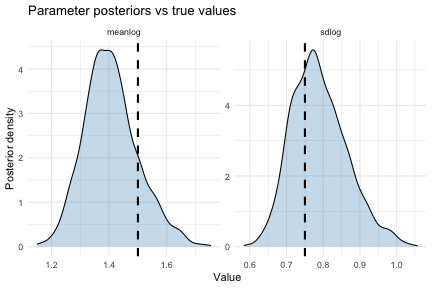

plot of chunk recovery-params

The dashed lines mark the true parameter values. The posteriors should concentrate around these values.

We can also compare the implied delay density from the posterior against the true distribution.

max_x <- max(delays) + 2
x_seq <- seq(0.01, max_x, length.out = 200)

set.seed(1)
draw_idx <- sample(length(post_meanlog), 100)
post_densities <- sapply(draw_idx, function(i) {
  dlnorm(x_seq, post_meanlog[i], post_sdlog[i])
})

plot_df <- data.frame(
  x = x_seq,
  true_density = dlnorm(
    x_seq, true_meanlog, true_sdlog
  ),
  post_median = apply(
    post_densities, 1, median
  ),
  post_lower = apply(
    post_densities, 1, quantile, 0.05
  ),
  post_upper = apply(
    post_densities, 1, quantile, 0.95
  )
)

ggplot(plot_df, aes(x = x)) +
  geom_ribbon(
    aes(ymin = post_lower, ymax = post_upper),
    fill = "#4292C6", alpha = 0.3
  ) +
  geom_line(
    aes(y = post_median, colour = "Fitted (posterior)")
  ) +
  geom_line(
    aes(y = true_density, colour = "True"),
    linetype = "dashed", linewidth = 1
  ) +
  scale_colour_manual(
    values = c(
      "Fitted (posterior)" = "#4292C6",
      "True" = "#252525"
    )
  ) +
  labs(
    x = "Delay (days)", y = "Density",
    colour = NULL,
    title = "Fitted vs true delay distribution"
  ) +
  theme_minimal() +
  theme(legend.position = "bottom")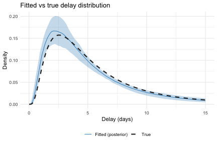

plot of chunk recovery-density

Note that get_parameters() returns Normal approximations to the marginal posteriors. The actual posterior may not be exactly normal. For full posterior access, use result$fit directly with extract_samples().

Charniga, K., Park, S. W., Akhmetzhanov, A. R., Cori, A., Dushoff, J., Funk, S., Gostic, K. M., Linton, N. M., Lison, A., Overton, C. E., Pulliam, J. R. C., Ward, T., Cauchemez, S., & Abbott, S. (2024). Best practices for estimating and reporting epidemiological delay distributions of infectious diseases. PLoS Comput. Biol., 20(10), e1012520. https://doi.org/10.1371/journal.pcbi.1012520