Model overview

Introduction

EpiNow2 provides several estimation models that can be combined for end-to-end epidemiological inference and forecasting. This vignette gives an overview of how these models connect. For a reference of what each model can do see the model features vignette.

Architecture

The diagram below shows the main functions and how they relate to one another.

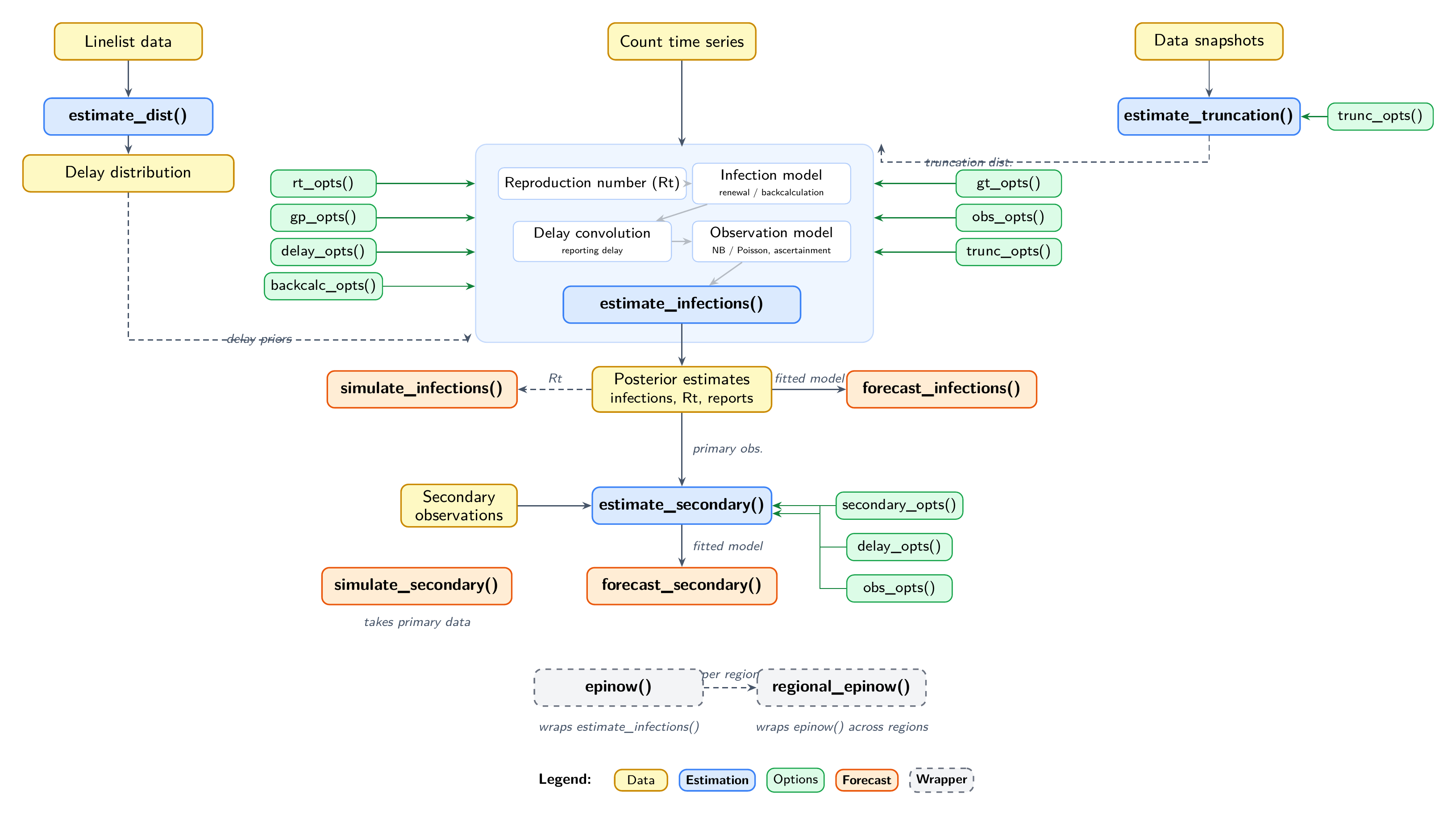
Data flows from top to bottom. Solid arrows show direct dependencies; dashed arrows show optional connections. Green boxes are options functions that configure the estimation models. See the model features vignette for what each function and option does.

Relationship between models

estimate_dist() fits delay distributions from linelist data, accounting for double interval censoring and right truncation. Its output can define priors for the other models via delay_opts(), gt_opts(), or trunc_opts().

estimate_truncation() produces both a nowcast and a truncation distribution from multiple snapshots of the same data. The distribution is typically passed to estimate_infections() via trunc_opts() for truncation-adjusted inference, but can also be used via delay_opts() or gt_opts() where appropriate.

estimate_infections() is the core model, estimating latent infections and the time-varying reproduction number from a count time series. Its posterior feeds into forecast_infections() for projections and can inform simulate_infections() for scenario analysis.

Estimated primary observations from estimate_infections() are used as input to estimate_secondary(), which estimates secondary outcomes (e.g. deaths, hospitalisations). forecast_secondary() extends a fitted secondary model with new primary data; simulate_secondary() generates synthetic secondary observations.

epinow() wraps estimate_infections() with logging and formatted output. regional_epinow() runs epinow() across regions in parallel.

Where to look next

Start here

• Getting started — quick introduction and basic usage
• Model features — feature reference for arguments and options

Model definitions (mathematical detail)

• Infection model — estimate_infections()
  • Gaussian process implementation — shared component used inside the renewal and back-calculation models
• Secondary model — estimate_secondary()
• Truncation model — estimate_truncation()
• Delay distribution fitting — estimate_dist()

Applied use

• Workflow — end-to-end estimation and forecasting
• Configuration examples — different model configurations with results
• Prior choice guide — default priors and how to modify them
• Production use — epinow() and regional_epinow()
• Case studies — external applications in the literature