National estimates
This page gives the national estimates from the joint model. The methods for this model are on the Methods page.
This page is generated from docs/pages/estimates/national.jl. The model code it calls is in src/. See aim and origins and limitations.
Offline copy. Each results release attaches the rendered site built from the same run: download the latest. The README.txt inside says how to view it.
Load packages, data and fitted chains
# Shared setup: packages, observations and the fit registry. See
# `docs/pages/_setup.jl`.
using BVDOutbreakSize
include(joinpath(pkgdir(BVDOutbreakSize), "docs", "pages", "_setup.jl"))
validation_forecast_from (generic function with 1 method)# The fits and prior draws this page reads, loaded from the cache here.
chn_joint = load_fit("joint")
chn_no_patches = load_fit("sens_no_patches")
chn_exports = load_fit("exports")
chn_deaths = load_fit("deaths")
chn_cases = load_fit("cases")
chn_confirmed = load_fit("confirmed")
chn_confirmed_deaths = load_fit("confirmed_deaths")
chn_treatment = load_fit("treatment")
chn_onsets = load_fit("onsets")
frozen_lastweek = load_fit("frozen_validation")
frozen_lastweek_streams = frozen_validation_stream_fits()
frozen_by_cutoff = frozen_fits_by_cutoff()
frozen_results = [frozen_by_cutoff[c] for c in frozen_cutoffs]
if RUN_SENSITIVITY
chn_joint_community_delay = load_fit("sens_community_delay")
chn_joint_exp_growth_clock = load_fit("sens_exp_growth_clock")
end
posterior_C_joint = vec(Array(chn_joint[:C_T]))
prior_chn = joint_prior_draws();Last updated: 30 September 2026.
Data as of: 26 September 2026.
Results
Summary
The numbers below are our estimate of the underlying infections to date, reported and unreported, from the joint posterior. Each is given as equal-tailed 30%, 60% and 90% credible intervals. The estimates for each province are on the province estimates page.
Compute the headline ranges
summary_ranges = let
    med(x) = quantile(x, 0.5)
    iqr(x) = quantile(x, 0.75) - quantile(x, 0.25)
    # Posterior-minus-prior shift in units of the parameter's prior IQR,
    # reusing the prior draws so nothing is respecified here.
    shift(post, prior) = round(
        (med(post) - med(prior)) / iqr(prior);
        digits = 2
    )

    C = posterior_C_joint
    Td = vec(Array(chn_joint[:T]))
    r0d = vec(Array(chn_joint[:r0]))
    rd = vec(Array(chn_joint[:r]))
    dt = vec(Array(chn_joint[:doubling_time]))
    R0d = vec(Array(chn_joint[:R0]))
    RTd = vec(Array(chn_joint[:R_T]))
    cfrd = vec(Array(chn_joint[:CFR]))
    sC = posterior_summary(C)
    sT = posterior_summary(Td)
    sr0 = posterior_summary(r0d)
    sr = posterior_summary(rd)
    # Doubling time is unbounded at zero growth, so its own quantiles do
    # not bound it once the growth rate spans zero. Map the growth rate's
    # interval instead, as the summary tables do.
    sdt0 = map(doubling_time, posterior_summary(r0d))
    sdt = map(doubling_time, posterior_summary(rd))
    sR0 = posterior_summary(R0d)
    sRT = posterior_summary(RTd)
    scfr = posterior_summary(cfrd)

    # The 30/60/90% interval phrase.
    ints(s, d) = BVDOutbreakSize._interval_text(s; digits = d)
    start_from(t) = obs.cutoff - Day(round(Int, t))
    ints_d(s) = string(
        "30% ", start_from(s.hi30), "–", start_from(s.lo30),
        ", 60% ", start_from(s.hi60), "–", start_from(s.lo60),
        ", 90% ", start_from(s.hi90), "–", start_from(s.lo90)
    )
    f_lo = round(sC.lo90 / obs.confirmed_cases; digits = 1)
    f_hi = round(sC.hi90 / obs.confirmed_cases; digits = 1)

    # How far the data has moved each estimate from its prior, in prior
    # interquartile ranges, reusing the prior draws.
    moves = [
        "cumulative infection count" => shift(C, vec(Array(prior_chn[:C_T]))),
        "outbreak age" => shift(Td, vec(Array(prior_chn[:T]))),
        "doubling time" => shift(dt, vec(Array(prior_chn[:doubling_time]))),
    ]
    biggest = argmax(p -> abs(p.second), moves)

    Markdown.parse(
        """
        - **Cumulative infections:** the outbreak is estimated to have caused
          $(ints(sC, 0)) infections to date, reported and unreported.
        - Against the $(obs.confirmed_cases) laboratory-confirmed cases by the
          cut-off that is roughly $(f_lo)–$(f_hi)× as many infections, so
          confirmed cases are estimated to capture only a small share of the
          outbreak.
        - **Outbreak start and age:** the outbreak is estimated to have begun on
          a start date of $(ints_d(sT)), an elapsed age to the cut-off of
          $(ints(sT, 0)) days.
        - **Growth rate and doubling time:** the initial growth rate is
          estimated to have been $(ints(sr0, 3)) per day, an initial doubling
          time of $(ints(sdt0, 1)) days.
          The latest growth rate is estimated to be $(ints(sr, 3)) per day, a
          latest doubling time of $(ints(sdt, 1)) days.
        - **Reproduction number:** the initial reproduction number is estimated
          to have been $(ints(sR0, 2)) and the latest to be $(ints(sRT, 2)).
        - **Case-fatality ratio:** the case-fatality ratio is estimated to be
          $(ints(scfr, 2)).
        - **Shift from priors:** how far the data has moved each estimate from
          its prior, in prior interquartile ranges, where a value of one means
          the posterior median sits one prior interquartile range from the prior
          median, zero means unchanged, and the sign gives the direction.
          The fit moves the cumulative infection count by $(moves[1].second),
          the outbreak age by $(moves[2].second) and the doubling time by
          $(moves[3].second); the largest move is in the $(biggest.first).
        """
    )
end;
Cumulative infections: the outbreak is estimated to have caused 30% 16593–20232, 60% 14887–22555, 90% 12343–27006 infections to date, reported and unreported.
Against the 8067 laboratory-confirmed cases by the cut-off that is roughly 1.5–3.3× as many infections, so confirmed cases are estimated to capture only a small share of the outbreak.
Outbreak start and age: the outbreak is estimated to have begun on a start date of 30% 2026-03-13–2026-03-20, 60% 2026-03-09–2026-03-24, 90% 2026-02-28–2026-03-28, an elapsed age to the cut-off of 30% 190–197, 60% 186–201, 90% 182–210 days.
Growth rate and doubling time: the initial growth rate is estimated to have been 30% 0.049–0.061, 60% 0.043–0.07, 90% 0.034–0.086 per day, an initial doubling time of 30% 14.1–11.3, 60% 16.0–9.9, 90% 20.1–8.1 days. The latest growth rate is estimated to be 30% -0.015–-0.003, 60% -0.022–0.004, 90% -0.037–0.017 per day, a latest doubling time of 30% -46.6–-199.0, 60% -31.2–191.5, 90% -19.0–41.0 days.
Reproduction number: the initial reproduction number is estimated to have been 30% 1.76–2.0, 60% 1.66–2.17, 90% 1.5–2.57 and the latest to be 30% 0.81–0.95, 60% 0.73–1.05, 90% 0.58–1.24.
Case-fatality ratio: the case-fatality ratio is estimated to be 30% 0.45–0.5, 60% 0.42–0.53, 90% 0.37–0.58.
Shift from priors: how far the data has moved each estimate from its prior, in prior interquartile ranges, where a value of one means the posterior median sits one prior interquartile range from the prior median, zero means unchanged, and the sign gives the direction. The fit moves the cumulative infection count by -0.06, the outbreak age by -1.25 and the doubling time by -1.19; the largest move is in the outbreak age.
Fit diagnostics
Fit diagnostics for the joint fit and each individual fit. These indicate how reliable the results are from the perspective of the inference algorithm. The breakdown by parameter can be used to further diagnose any issues.
Build the fit diagnostics table
fit_diagnostics_table = diagnostics_table(
    "joint" => chn_joint,
    "joint, no patches" => chn_no_patches,
    "exports" => chn_exports,
    "deaths (DRC)" => chn_deaths,
    "cases (DRC)" => chn_cases,
    "confirmed (DRC)" => chn_confirmed,
    "confirmed deaths (DRC)" => chn_confirmed_deaths,
    "isolation (DRC)" => chn_treatment,
    "onsets (DRC)" => chn_onsets,
    "frozen (1wk back)" => frozen_lastweek.chn,
    (
        RUN_SENSITIVITY ?
            [
                "delay sensitivity" => chn_joint_community_delay,
                "clock sensitivity (ExpGrowth)" => chn_joint_exp_growth_clock,
            ] :
            []
    )...
);

# Only the joint fit is held to the convergence thresholds.
include(joinpath(pkgdir(BVDOutbreakSize), "docs", "fits", "convergence.jl"))
fit_convergence_summary = convergence_summary(
    "joint", fit_diagnostics(chn_joint)
)
fit_diagnostics_detail_md = let t = fit_diagnostics_table,
        rhat = filter(r -> isfinite(r.max_rhat), t),
        ess = filter(r -> isfinite(r.min_ess_bulk), t),
        worst = rhat[argmax(rhat.max_rhat), :],
        least = ess[argmin(ess.min_ess_bulk), :]

    fit_convergence_summary.detail * "\n\n" *
        "Across all $(size(t, 1)) fits the worst R-hat is " *
        "$(fmt_value(worst.max_rhat)), in the $(worst.fit) fit. " *
        "The lowest bulk effective sample size is " *
        "$(fmt_count(least.min_ess_bulk)), in the $(least.fit) fit. " *
        "Only the joint fit is held to the thresholds above."
end
fit_diagnostics_detail = Markdown.parse(fit_diagnostics_detail_md);
The joint fit passes the convergence checks with warnings.
Fit diagnostics table
Its worst R-hat is 1.06 and its lowest bulk effective sample size is 49, with 2 divergent transitions in 2000 draws. A fit passes without warnings when its worst R-hat is at most 1.05, its effective sample sizes are at least 100 and at most 1% of its draws diverge.
Across all 10 fits the worst R-hat is 1.85, in the frozen (1wk back) fit. The lowest bulk effective sample size is 6, in the frozen (1wk back) fit. Only the joint fit is held to the thresholds above.
| Row | fit | max_rhat | min_ess_bulk | divergences |
|---|---|---|---|---|
| String | Float64 | Float64 | Int64 | |
| 1 | joint | 1.062 | 49.0 | 2 |
| 2 | joint, no patches | 1.022 | 73.0 | 0 |
| 3 | exports | 1.02 | 475.0 | 0 |
| 4 | deaths (DRC) | 1.014 | 268.0 | 1 |
| 5 | cases (DRC) | 1.012 | 496.0 | 0 |
| 6 | confirmed (DRC) | 1.01 | 352.0 | 11 |
| 7 | confirmed deaths (DRC) | 1.015 | 491.0 | 2 |
| 8 | isolation (DRC) | 1.015 | 173.0 | 2 |
| 9 | onsets (DRC) | 1.123 | 16.0 | 0 |
| 10 | frozen (1wk back) | 1.847 | 6.0 | 1 |
Data currency
The cut-off is the last date any stream reports.
Build the data currency table
stream_status = stream_report_status(obs)
stream_currency_table = let stale = stream_status[.!stream_status.reporting, :]
    DataFrame(
        "Stream" => stale.label,
        "Last reported" => [
            ismissing(d) ? "never" : string(d) for d in stale.last_date
        ],
        "Days before cut-off" => [
            ismissing(d) ? "-" : string(d) for d in stale.days_since
        ]
    )
end
stream_currency_summary = let n = length(stream_status.stream),
        n_current = count(stream_status.reporting),
        cutoff = format_report_date(obs.cutoff)

    Markdown.parse(
        if n_current == n
            "All $n streams report within " *
                "$(STREAM_REPORTING_GRACE_DAYS) days of the $cutoff cut-off."
        else
            "$n_current of the $n streams report within " *
                "$(STREAM_REPORTING_GRACE_DAYS) days of the $cutoff cut-off. " *
                "The other $(n - n_current) stopped earlier and are " *
                "carried frozen."
        end
    )
end;
13 of the 25 streams report within 7 days of the 26 September 2026 cut-off. The other 12 stopped earlier and are carried frozen.
Streams that stop before the cut-off
| Stream | Last reported | Days before cut-off |
|---|---|---|
| Suspected cases | 2026-05-26 | 123 |
| Suspected deaths | 2026-05-26 | 123 |
| New suspected deaths/day | 2026-07-11 | 77 |
| Specimens analysed (cumulative) | 2026-05-28 | 121 |
| Specimens received | 2026-05-28 | 121 |
| Admissions/day | 2026-08-02 | 55 |
| In-care deaths/day | 2026-08-02 | 55 |
| Rule-outs/day | 2026-08-02 | 55 |
| Absconded/day | 2026-08-02 | 55 |
| Confirmed in care | 2026-08-02 | 55 |
| Suspects in care | 2026-08-02 | 55 |
| Uganda exports | 2026-05-23 | 126 |
Joint model estimates
Cumulative infection count summary table
cumulative_cases_summary = summary_table(
    chn_joint, [:C_T]; digits = 0
);| Row | Quantity | Lower 90% | Lower 60% | Lower 30% | Upper 30% | Upper 60% | Upper 90% |
|---|---|---|---|---|---|---|---|
| String | Float64 | Float64 | Float64 | Float64 | Float64 | Float64 | |
| 1 | C_T | 12343.0 | 14887.0 | 16593.0 | 20232.0 | 22555.0 | 27006.0 |
The figure below shows the cumulative trajectories and current-cut-off densities for three latent quantities: infections, symptom onsets and deaths. The infection density is the headline outbreak size, a count of infections rather than reported cases.
Cumulative infections, onsets and deaths figure
cumulative_traj_fig = plot_cumulative_trajectories(
    chn_joint;
    n = obs.n, seeding = obs.seeding
);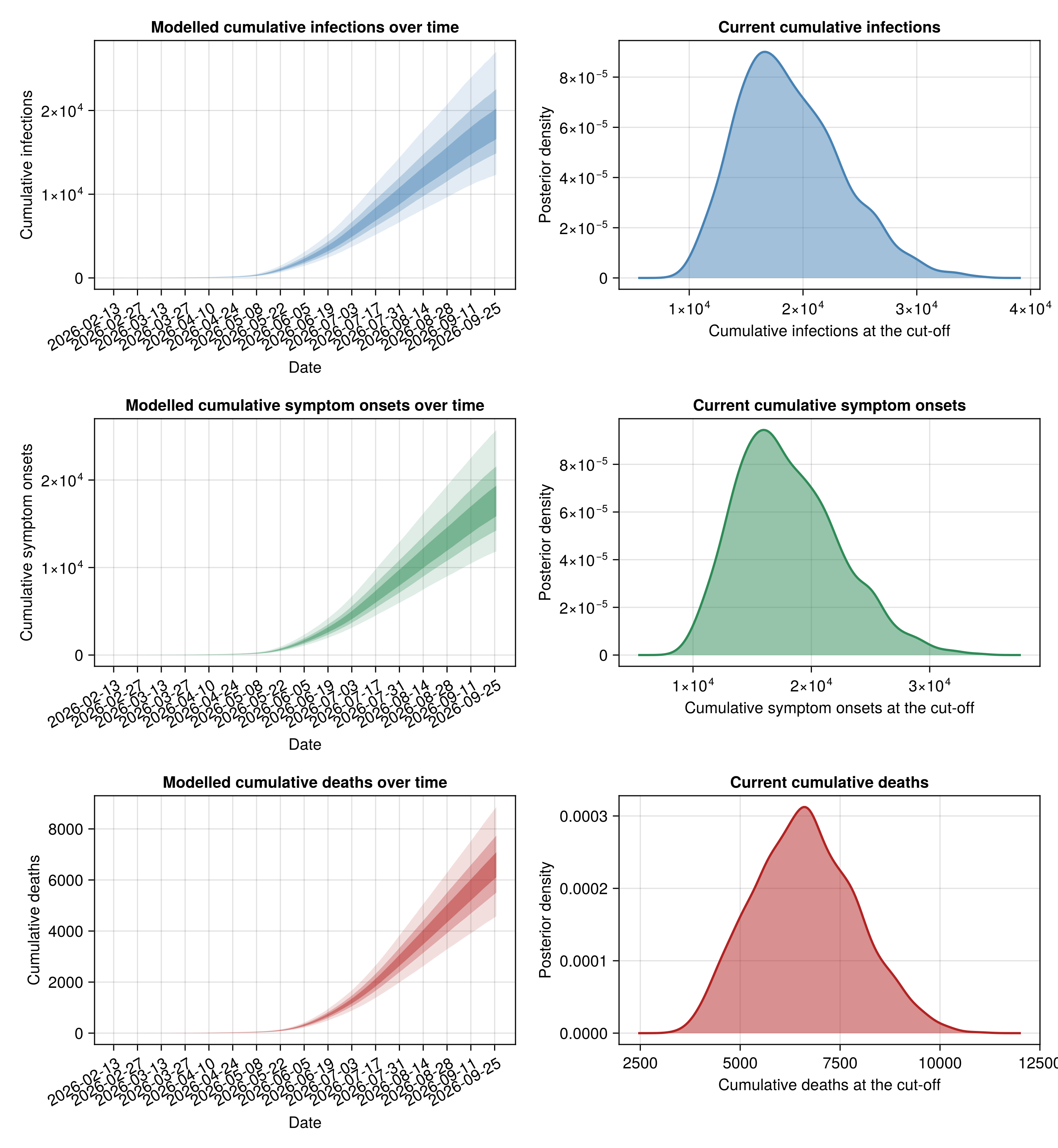
The national count above is the sum of the four patches' renewal equations. The per-province sizes, the modelled infections behind them and the importation between provinces are on the province estimates page.
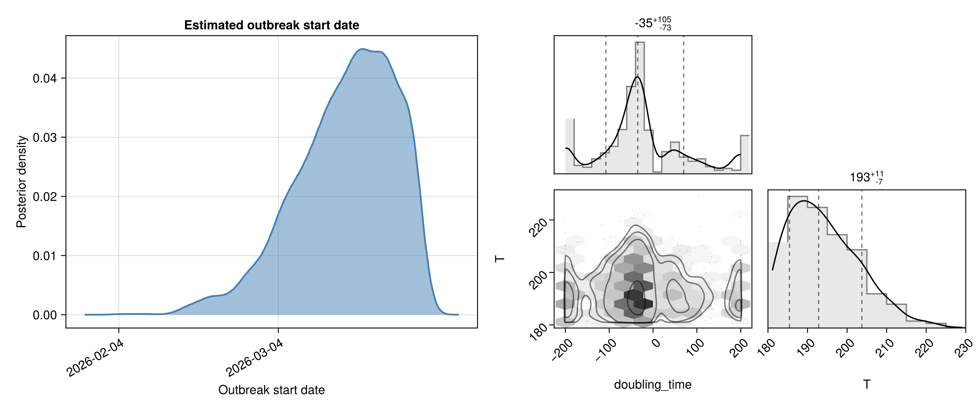
The cumulative infection count is set by the reproduction number trajectory and the outbreak age. The left panel below shows the posterior for the outbreak start date. The right panel shows the joint posterior of the outbreak age and the early doubling time.
Outbreak start date and seeding-time posterior
start_date_fig = plot_start_date_pair(
    chn_joint;
    as_of_date = string(obs.cutoff)
);
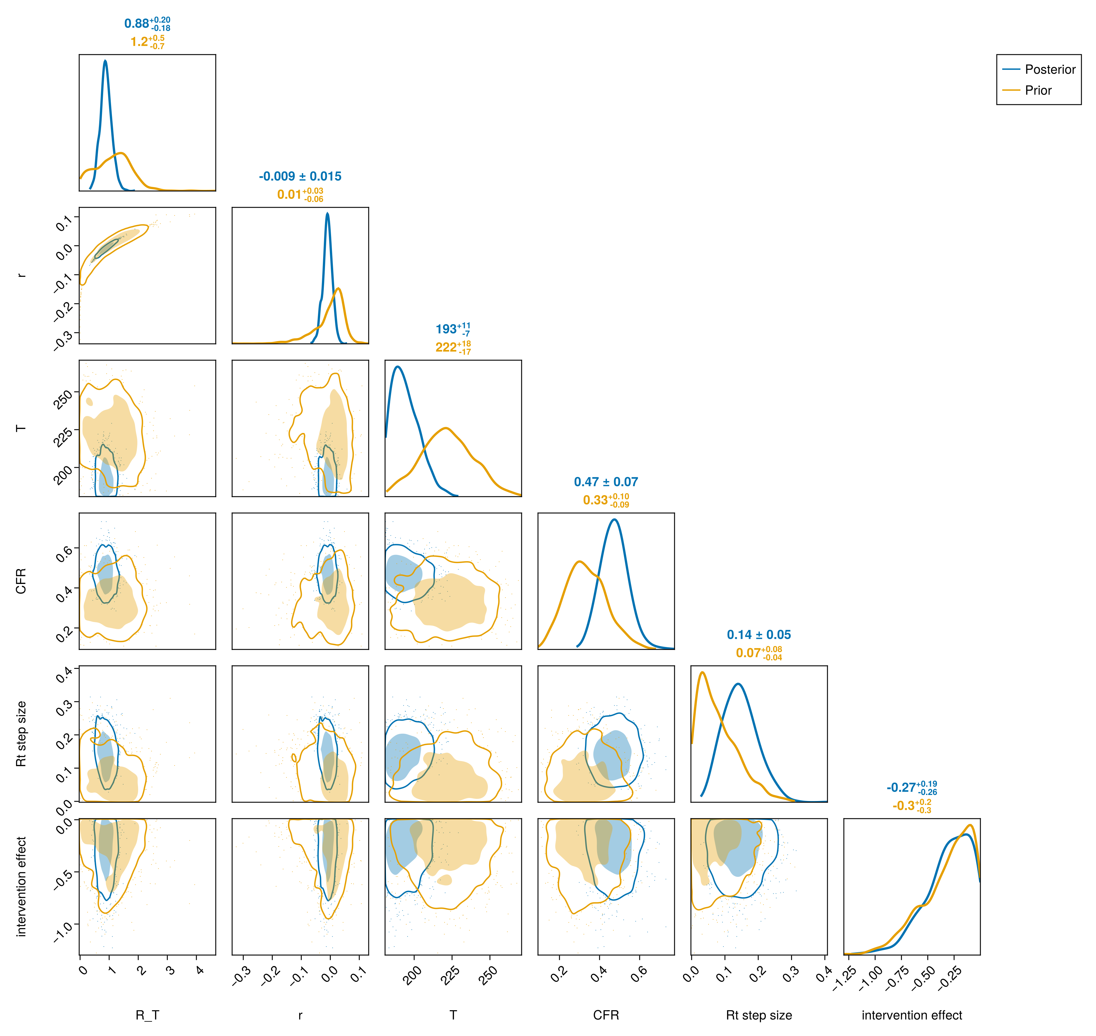
The table below reports credible intervals on the infection-process parameters: the growth rate and doubling time, the reproduction number, the outbreak age, the case-fatality ratio and the cumulative infection count. The pair plot beside it shows their joint posterior, with the prior overlaid so the data's contribution to each marginal is visible.
Infection-parameter summary table
infection_summary = summary_table(
    chn_joint,
    [:r, :doubling_time, :T, :R_T, :CFR, :C_T]; digits = 2
);| Row | Quantity | Lower 90% | Lower 60% | Lower 30% | Upper 30% | Upper 60% | Upper 90% |
|---|---|---|---|---|---|---|---|
| String | Float64 | Float64 | Float64 | Float64 | Float64 | Float64 | |
| 1 | r | -0.04 | -0.02 | -0.01 | -0.0 | 0.0 | 0.02 |
| 2 | doubling_time | -18.98 | -31.17 | -46.55 | -199.04 | 191.51 | 40.96 |
| 3 | T | 182.32 | 186.2 | 189.6 | 196.56 | 201.32 | 210.13 |
| 4 | R_T | 0.58 | 0.73 | 0.81 | 0.95 | 1.05 | 1.24 |
| 5 | CFR | 0.37 | 0.42 | 0.45 | 0.5 | 0.53 | 0.58 |
| 6 | C_T | 12343.3 | 14886.5 | 16593.5 | 20232.0 | 22554.5 | 27005.5 |
Infection-parameter pair plot (prior overlaid)
infection_pair_fig = plot_pair(
    chn_joint,
    [
        :R_T, :r, :T, :CFR,
        Symbol("rt_state.sigma_rw"), Symbol("rt_state.intervention_effect"),
    ];
    prior = prior_chn, labels = display_names
);
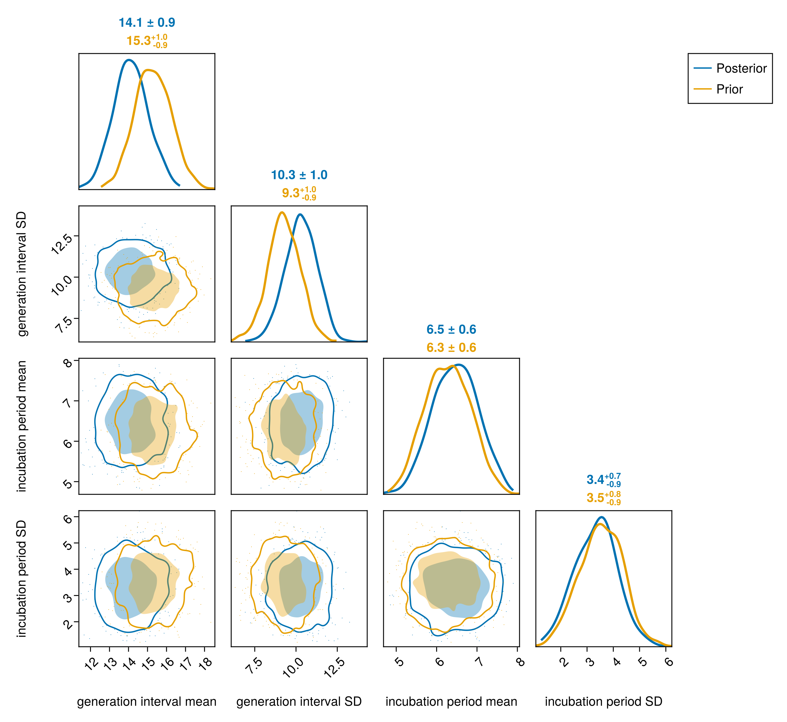
The infection model carries two delays: the generation interval and the incubation period. The table and pair plot below report their posterior means and standard deviations.
Infection-delay summary table
infection_delay_summary = summary_table(
    chn_joint,
    [
        Symbol("gi_state.gi_mean"), Symbol("gi_state.gi_sd"),
        Symbol("inc_state.delay_mean"), Symbol("inc_state.delay_sd"),
    ];
    digits = 2, labels = display_names
);
Show infection-delay summary table
| Row | Quantity | Lower 90% | Lower 60% | Lower 30% | Upper 30% | Upper 60% | Upper 90% |
|---|---|---|---|---|---|---|---|
| String | Float64 | Float64 | Float64 | Float64 | Float64 | Float64 | |
| 1 | generation interval mean | 12.62 | 13.38 | 13.78 | 14.47 | 14.88 | 15.71 |
| 2 | generation interval SD | 8.68 | 9.51 | 9.96 | 10.69 | 11.1 | 11.84 |
| 3 | incubation period mean | 5.56 | 6.0 | 6.26 | 6.71 | 6.95 | 7.38 |
| 4 | incubation period SD | 1.98 | 2.65 | 3.04 | 3.66 | 4.01 | 4.62 |
Infection-delay pair plot (prior overlaid)
infection_delay_pair_fig = plot_pair(
    chn_joint,
    [
        Symbol("gi_state.gi_mean"), Symbol("gi_state.gi_sd"),
        Symbol("inc_state.delay_mean"), Symbol("inc_state.delay_sd"),
    ];
    prior = prior_chn, labels = display_names
);
Reproduction number over time
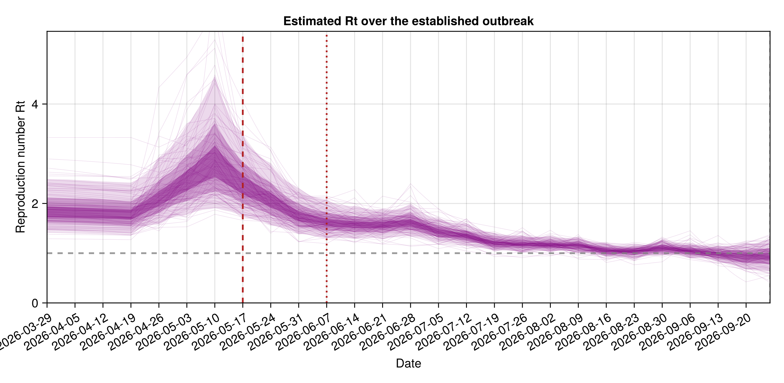
The figure below shows the daily reproduction number over the established outbreak, from the genetic bound to the cut-off. The 30%, 60% and 90% credible ribbons are shown with about a hundred sampled trajectories, and the no-growth threshold at one as a grey dashed line. The first situation report on 18 May 2026 marks the start of the response scale-up (red dashed). The end of the three-week scale-up is the red dotted line, and the data cut-off is grey dashed.
Reproduction-number trajectory
# `rt_start` is the renewal/established-window start the plot shows from;
# `rt_walk_start` is where the random walk's knots begin — `RT_WALK_LEAD`
# days (a month) before the first situation report, matching `bvd_joint`'s
# `rt_walk_lead` — so the chain reconstruction uses the same knot grid the
# model did, floored at the renewal start. R_t is flat at R0 between the two.
rt_fig = plot_rt(
    chn_joint;
    n = obs.n, breakpoint = _BREAKPOINT,
    rt_start = _rt_start_plot,
    rt_walk_start = clamp(_BREAKPOINT - RT_WALK_LEAD, _rt_start_plot, obs.n),
    as_of_date = string(obs.cutoff), seeding = obs.seeding,
    ramp = RT_INTERVENTION_RAMP
);
The same trajectory split by province, the per-province summary and the spatial hyperparameters are on the province estimates page.
The table reports the posterior of the response effect on the reproduction number as a multiplier, where a value below one is the factor by which the response lowers the reproduction number once the scale-up completes.
Intervention-effect summary table
intervention_effect = vec(
    Array(
        chn_joint[Symbol("rt_state.intervention_effect")]
    )
);
intervention_table = streams_table(
    "Rt multiplier exp(effect)" => exp.(intervention_effect);
    digits = 2
);| Row | Stream | Lower 90% | Lower 60% | Lower 30% | Upper 30% | Upper 60% | Upper 90% |
|---|---|---|---|---|---|---|---|
| String | Float64 | Float64 | Float64 | Float64 | Float64 | Float64 | |
| 1 | Rt multiplier exp(effect) | 0.5 | 0.62 | 0.71 | 0.84 | 0.91 | 0.98 |
Observation delays
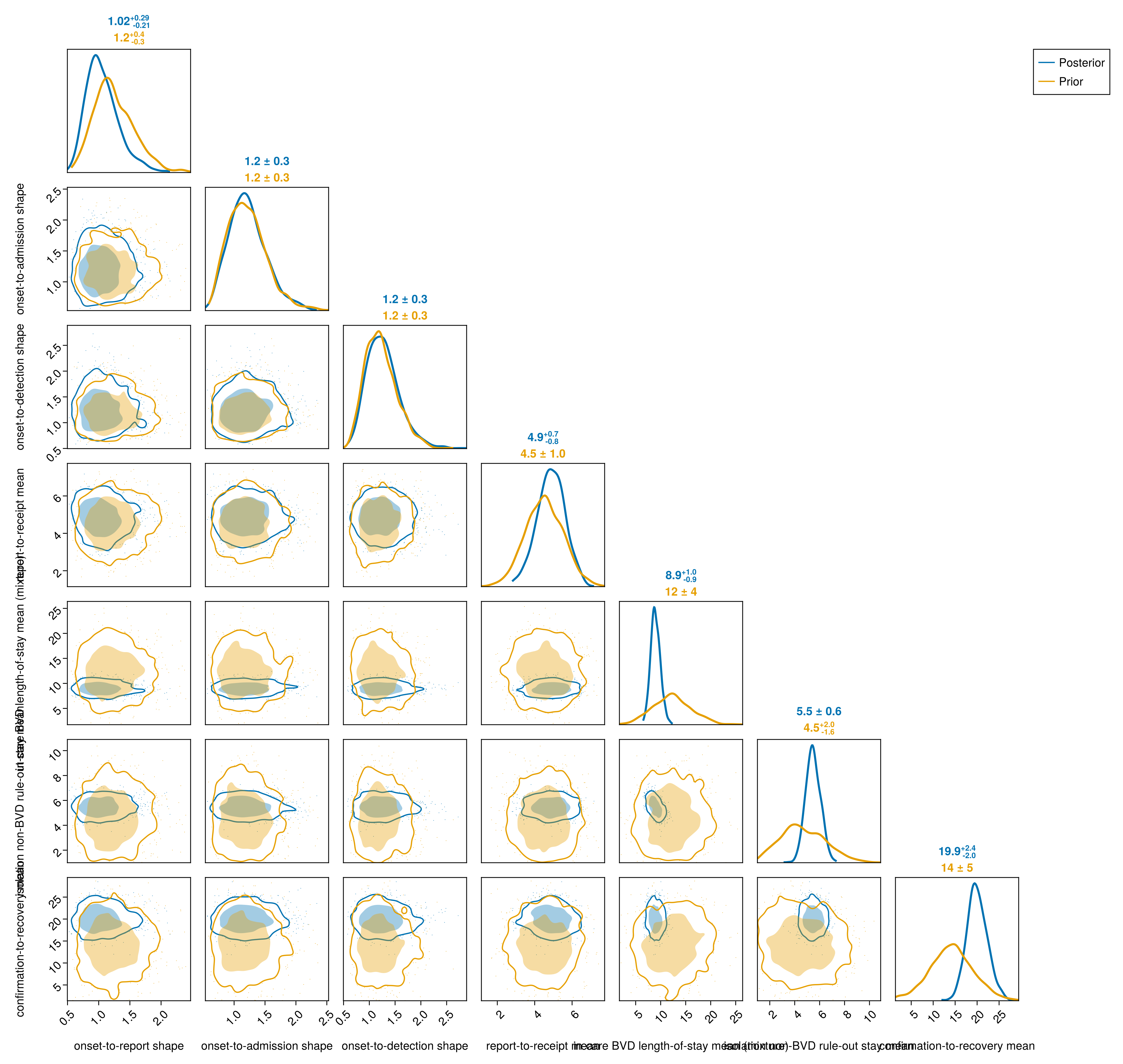
The delays carry latent infections through to each observed event: reporting, death, hospitalisation abroad and laboratory receipt. The onset-to-report and onset-to-hospitalisation delays are the same line-list onset-to-admission delay, sampled on its natural Gamma shape and scale. The onset-to-death delay is the convolution of two atomic Gamma delays, onset-to-admission and admission-to-death, each with its own shape and scale. The report-to-receipt delay is sampled by its mean and standard deviation. The length-of-stay delays are also shown: the isolation-bed BVD treatment stay (prior: the line-list admission-to-death delay), the non-BVD rule-out stay (prior: the report-to-receipt turnaround), and the confirmation-to-recovery delay.
Observation-delay summary table
obs_delay_summary = summary_table(
    chn_joint,
    [
        Symbol("cases_state.report_state.α"),
        Symbol("cases_state.report_state.θ"),
        Symbol("deaths_state.od_state.oa.α"),
        Symbol("deaths_state.od_state.oa.θ"),
        Symbol("deaths_state.od_state.ad.α"),
        Symbol("deaths_state.od_state.ad.θ"),
        Symbol("exports_state.detect_state.α"),
        Symbol("exports_state.detect_state.θ"),
        Symbol("confirmed_state.receipt_state.d.delay_mean"),
        Symbol("confirmed_state.receipt_state.d.delay_sd"),
        :isolation_bvd_los_mean,
        :isolation_ruleout_los_mean,
        :recovery_delay_mean,
    ];
    digits = 2, labels = display_names
);
Show observation-delay summary table
| Row | Quantity | Lower 90% | Lower 60% | Lower 30% | Upper 30% | Upper 60% | Upper 90% |
|---|---|---|---|---|---|---|---|
| String | Float64 | Float64 | Float64 | Float64 | Float64 | Float64 | |
| 1 | onset-to-report shape | 0.71 | 0.84 | 0.94 | 1.13 | 1.26 | 1.55 |
| 2 | onset-to-report scale | 1.13 | 1.65 | 2.05 | 2.76 | 3.24 | 4.11 |
| 3 | onset-to-admission shape | 0.78 | 0.96 | 1.08 | 1.3 | 1.45 | 1.76 |
| 4 | onset-to-admission scale | 1.88 | 2.9 | 3.52 | 4.46 | 4.98 | 5.88 |
| 5 | admission-to-death shape | 1.26 | 1.73 | 1.96 | 2.34 | 2.55 | 2.97 |
| 6 | admission-to-death scale | 2.49 | 3.45 | 3.94 | 4.83 | 5.39 | 6.27 |
| 7 | onset-to-detection shape | 0.83 | 1.0 | 1.12 | 1.36 | 1.51 | 1.83 |
| 8 | onset-to-detection scale | 2.0 | 2.79 | 3.32 | 4.22 | 4.66 | 5.56 |
| 9 | report-to-receipt mean | 3.58 | 4.25 | 4.61 | 5.16 | 5.48 | 6.05 |
| 10 | report-to-receipt SD | 2.82 | 3.32 | 3.65 | 4.23 | 4.54 | 5.1 |
| 11 | in-care BVD length-of-stay mean (mixture) | 7.44 | 8.17 | 8.56 | 9.3 | 9.76 | 10.66 |
| 12 | isolation non-BVD rule-out stay mean | 4.54 | 4.99 | 5.25 | 5.67 | 5.97 | 6.46 |
| 13 | confirmation-to-recovery mean | 16.38 | 18.22 | 19.16 | 20.85 | 21.98 | 24.0 |
Observation-delay pair plot (prior overlaid)
obs_delay_pair_fig = plot_pair(
    chn_joint,
    [
        Symbol("cases_state.report_state.α"),
        Symbol("deaths_state.od_state.oa.α"),
        Symbol("exports_state.detect_state.α"),
        Symbol("confirmed_state.receipt_state.d.delay_mean"),
        :isolation_bvd_los_mean,
        :isolation_ruleout_los_mean,
        :recovery_delay_mean,
    ];
    prior = prior_chn, labels = display_names
);
Surveillance parameters
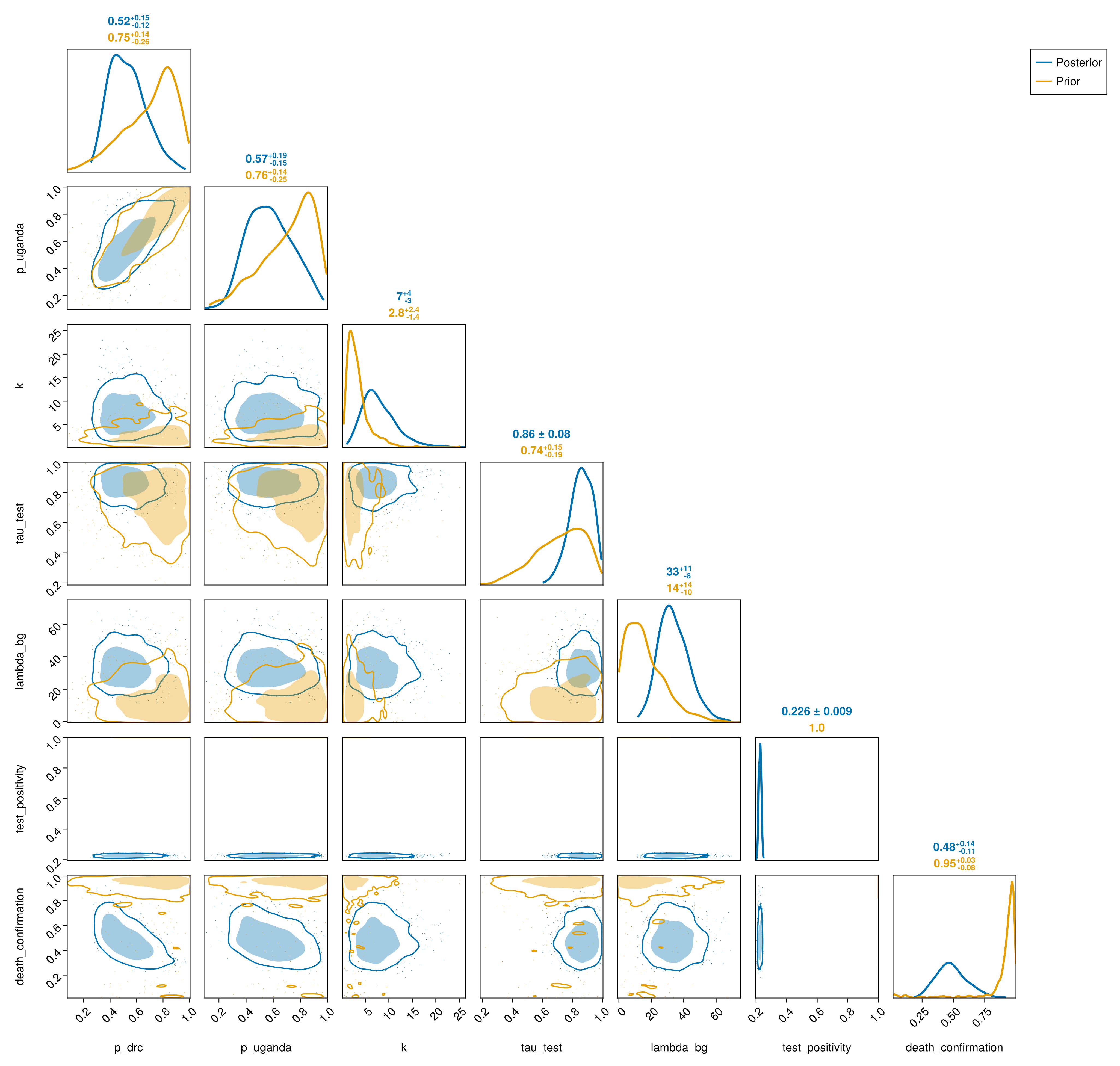
The surveillance-data parameters cover the reporting fractions for the DRC and Uganda, the surveillance dispersions, and the laboratory pipeline: the testing fraction and receipt delay, the specimens analysed per suspect sampled, the per-suspected and per-test positivity, the non-BVD background rate, and the death-confirmation probability. The six passive-surveillance count streams (suspected cases, suspected deaths, confirmed cases, confirmed deaths, isolation occupancy and recovered) each have their own negative-binomial dispersion, partially pooled from a shared population.
Surveillance-parameter summary table
surveillance_summary = summary_table(
    chn_joint,
    [
        :p_drc, :p_uganda, :k, :k_cases, :k_deaths, :k_confirmed,
        :k_confirmed_deaths, :dispersion_sd, :tau_test,
        :specimens_per_suspect, :lambda_bg,
        :suspected_positivity, :test_positivity, :expected_confirmed_T,
        :expected_analysed_T, :death_ascertainment, :background_cfr,
        :tau_death, :death_composition,
        :death_confirmation, :expected_confirmed_deaths_T,
        :isolation_admission, :isolation_dispersion, :expected_isolation_T,
        :expected_bed_demand_T, :bed_capacity, :bed_shortfall_T,
        :incare_cfr, :incare_cfr_modifier, :incare_confirm_modifier,
        :isolation_death_los_mean,
        :isolation_recovery_los_mean, :abscond_fraction,
        :recovery_probability, :recovered_dispersion, :expected_recovered_T,
    ];
    digits = 3
);
Show surveillance-parameter summary table
| Row | Quantity | Lower 90% | Lower 60% | Lower 30% | Upper 30% | Upper 60% | Upper 90% |
|---|---|---|---|---|---|---|---|
| String | Float64 | Float64 | Float64 | Float64 | Float64 | Float64 | |
| 1 | p_drc | 0.346 | 0.413 | 0.461 | 0.579 | 0.649 | 0.783 |
| 2 | p_uganda | 0.343 | 0.431 | 0.5 | 0.64 | 0.731 | 0.869 |
| 3 | k | 3.241 | 5.05 | 6.188 | 8.755 | 10.716 | 14.771 |
| 4 | k_cases | 8.851 | 9.932 | 10.645 | 11.965 | 12.868 | 14.368 |
| 5 | k_deaths | 6.533 | 8.124 | 9.262 | 11.365 | 12.957 | 16.483 |
| 6 | k_confirmed | 5.913 | 6.595 | 7.101 | 7.936 | 8.49 | 9.436 |
| 7 | k_confirmed_deaths | 5.581 | 6.736 | 7.47 | 8.896 | 9.848 | 11.863 |
| 8 | dispersion_sd | 0.411 | 0.503 | 0.578 | 0.721 | 0.826 | 1.07 |
| 9 | tau_test | 0.724 | 0.795 | 0.833 | 0.892 | 0.926 | 0.968 |
| 10 | specimens_per_suspect | 1.123 | 1.198 | 1.249 | 1.347 | 1.408 | 1.549 |
| 11 | lambda_bg | 19.913 | 26.05 | 29.648 | 36.892 | 41.301 | 51.397 |
| 12 | suspected_positivity | 0.206 | 0.218 | 0.227 | 0.243 | 0.255 | 0.284 |
| 13 | test_positivity | 0.213 | 0.218 | 0.222 | 0.229 | 0.233 | 0.24 |
| 14 | expected_confirmed_T | 8153.89 | 8373.42 | 8520.43 | 8784.0 | 8937.66 | 9200.12 |
| 15 | expected_analysed_T | 37504.3 | 38579.5 | 39188.3 | 40176.6 | 40786.8 | 41820.3 |
| 16 | death_ascertainment | 0.798 | 0.853 | 0.876 | 0.912 | 0.93 | 0.953 |
| 17 | background_cfr | 0.082 | 0.141 | 0.177 | 0.236 | 0.271 | 0.328 |
| 18 | tau_death | 0.465 | 0.525 | 0.57 | 0.654 | 0.716 | 0.853 |
| 19 | death_composition | 0.301 | 0.381 | 0.441 | 0.548 | 0.62 | 0.763 |
| 20 | death_confirmation | 0.301 | 0.38 | 0.431 | 0.523 | 0.589 | 0.715 |
| 21 | expected_confirmed_deaths_T | 3422.56 | 3533.86 | 3599.55 | 3706.49 | 3769.27 | 3878.97 |
| 22 | isolation_admission | 0.278 | 0.289 | 0.296 | 0.308 | 0.316 | 0.332 |
| 23 | isolation_dispersion | 102.96 | 116.276 | 125.722 | 142.75 | 154.85 | 176.272 |
| 24 | expected_isolation_T | 756.037 | 784.704 | 800.337 | 826.534 | 843.846 | 871.407 |
| 25 | expected_bed_demand_T | 834.369 | 880.249 | 905.581 | 944.855 | 967.699 | 1007.98 |
| 26 | bed_capacity | 1535.0 | 1535.0 | 1535.0 | 1535.0 | 1540.81 | 1582.06 |
| 27 | bed_shortfall_T | 0.0 | 1.227 | 3.073 | 6.163 | 7.998 | 11.92 |
| 28 | incare_cfr | 0.394 | 0.416 | 0.43 | 0.456 | 0.474 | 0.506 |
| 29 | incare_cfr_modifier | -0.595 | -0.356 | -0.217 | 0.01 | 0.133 | 0.349 |
| 30 | incare_confirm_modifier | 0.461 | 0.553 | 0.622 | 0.767 | 0.892 | 1.117 |
| 31 | isolation_death_los_mean | 2.88 | 4.516 | 5.433 | 7.209 | 8.315 | 10.556 |
| 32 | isolation_recovery_los_mean | 7.244 | 9.061 | 10.02 | 11.765 | 12.753 | 14.585 |
| 33 | abscond_fraction | 0.009 | 0.01 | 0.01 | 0.011 | 0.012 | 0.012 |
| 34 | recovery_probability | 0.267 | 0.283 | 0.292 | 0.307 | 0.317 | 0.337 |
| 35 | recovered_dispersion | 5.13 | 5.97 | 6.537 | 7.705 | 8.459 | 9.88 |
| 36 | expected_recovered_T | 1967.69 | 2035.92 | 2077.26 | 2147.25 | 2187.24 | 2270.65 |
Surveillance-parameter pair plot (prior overlaid)
surveillance_pair_fig = plot_pair(
    chn_joint,
    [
        :p_drc, :p_uganda, :k, :tau_test, :lambda_bg, :test_positivity,
        :death_confirmation,
    ];
    prior = prior_chn
);
Model against observed
Whether the fit reproduces the data it was fitted to, stream by stream, is on the in-sample checks page.
Symptom-onset reporting delay and ascertainment
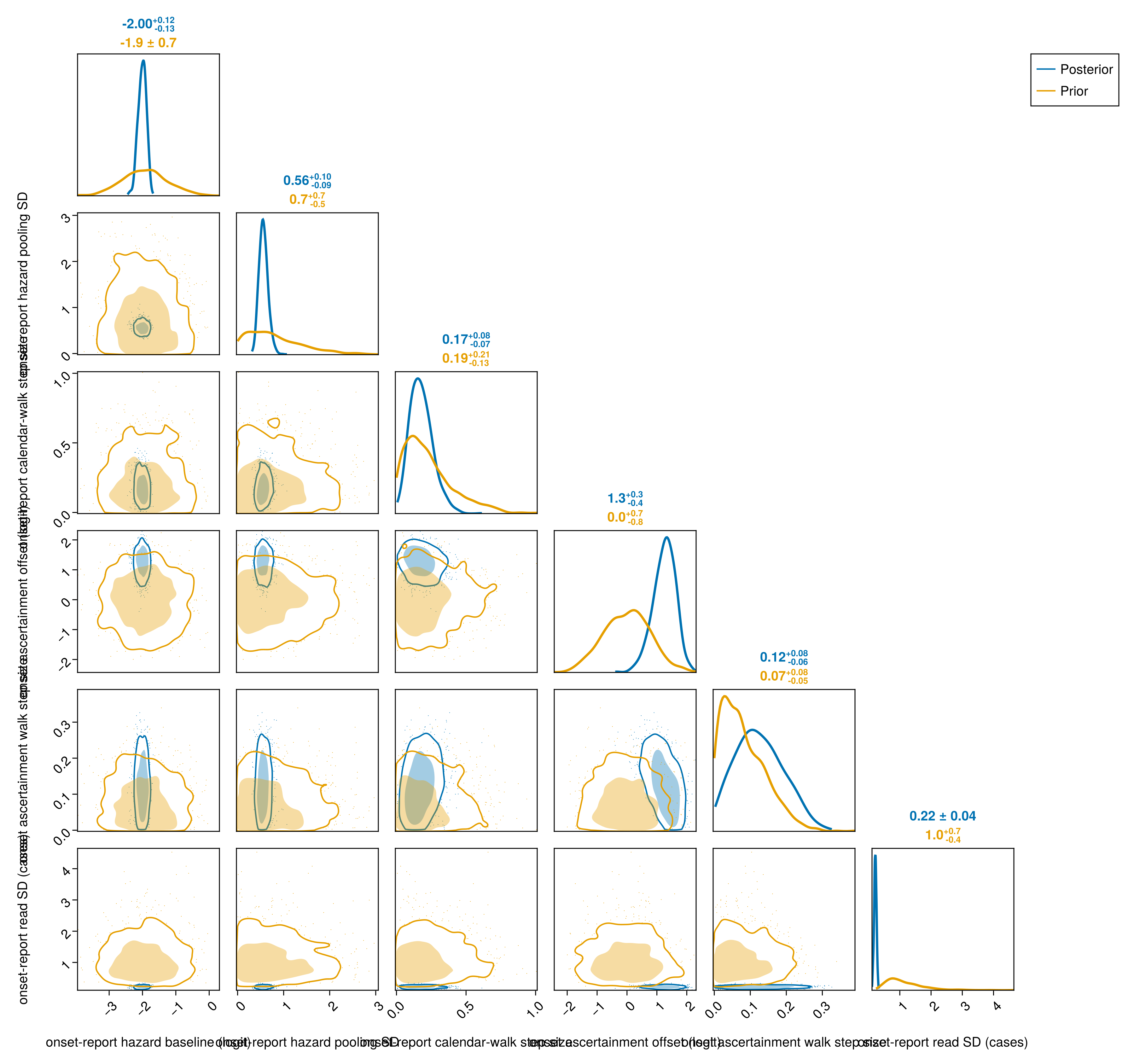
The table reports the onset-report hazard's hyperparameters and two derived quantities. These are the share of a representative onset date's eventual reports that arrive within 7 days, and the median modelled ascertainment over the onset dates the ascertainment walk spans. The first comes from the delay hazard and the second from the ascertainment level anchored on the confirmed pipeline, so they are separate estimates (see the symptom-onset reporting delay Methods section). The ascertainment offset is the row to read first, since it is the triangle's departure from the confirmed pipeline's own ascertainment and its prior is centred on no departure at all. The read SD row is the error the fit attributes to one digitised bar, in cases, on top of the rounding every integer read carries.
Reconstruct the onset-report hazard and calendar walk
# The report-date grid the calendar walk spans, `_onset_grid_start` to
# `_onset_grid_end`, is a fixed function of the digitised triangle rather
# than chain contents, so the shared setup builds it once from
# `obs.onset_curve_history`.
# Every posterior draw's `logit_h0` (the baseline delay hazard), `γ` (the
# report-date calendar walk) and ascertainment level, read off the fitted
# model's own onset-reporting state at each draw.
_onset_hazard = fitted_onset_hazard(fit_model("joint"), chn_joint)

# A representative onset day (the median scored onset date), so the 7-day
# fraction below reflects a typical, not an edge, calendar day.
_onset_u_ref = isempty(obs.onset_curve_history.onset_days) ?
    _onset_grid_start :
    round(Int, quantile(obs.onset_curve_history.onset_days, 0.5))
# The delay profile is the normalised delay CDF, which reaches one by
# construction, so the 7-day fraction is read straight off it.
_onset_7d_fraction = [
    onset_report_G(
        6, _onset_hazard.logit_h0[i],
        _onset_hazard.γ[i], _onset_u_ref,
        _onset_grid_start
    )
        for i in eachindex(_onset_hazard.logit_h0)
]
filter!(isfinite, _onset_7d_fraction)

# Per-draw median ascertainment over the onset dates the ascertainment
# walk spans, then summarised across draws. Ascertainment is its own
# level rather than the delay hazard's asymptote (see the [symptom-onset
# reporting delay](@ref "Symptom-onset reporting delay") Methods section).
_onset_ascertainment_draws = [
    quantile(_onset_hazard.alpha[i], 0.5)
        for i in eachindex(_onset_hazard.alpha)
]

_onset_labels = merge(
    display_names,
    Dict(
        Symbol("onset_report_state.η0") => "onset-report hazard baseline (logit)",
        Symbol("onset_report_state.σ_h0") => "onset-report hazard pooling SD",
        Symbol("onset_report_state.σ_γ") => "onset-report calendar-walk step size",
        Symbol("onset_report_state.β") => "onset ascertainment offset (logit)",
        Symbol("onset_report_state.σ_a") => "onset ascertainment walk step size",
        Symbol("onset_report_state.τ") => "onset-report read SD (cases)"
    )
);
Symptom-onset reporting-delay summary table
# Derived-quantity rows built with the same pre-prettify column schema
# `summary_table` uses, so they `vcat` cleanly onto its output.
onset_derived_raw = DataFrame(
    quantity = String[],
    lower_90 = Float64[], lower_60 = Float64[],
    lower_30 = Float64[], upper_30 = Float64[],
    upper_60 = Float64[], upper_90 = Float64[]
)
for (label, draws) in [
        (
            "share of eventual reports arriving within 7 days (median onset date)",
            _onset_7d_fraction,
        ),
        ("median modelled ascertainment", _onset_ascertainment_draws),
    ]
    s = posterior_summary(draws)
    push!(
        onset_derived_raw,
        (
            label, round(s.lo90; digits = 3), round(s.lo60; digits = 3),
            round(s.lo30; digits = 3), round(s.hi30; digits = 3),
            round(s.hi60; digits = 3), round(s.hi90; digits = 3),
        )
    )
end
onset_derived_table = BVDOutbreakSize._prettify(onset_derived_raw)

onset_summary = vcat(
    summary_table(
        chn_joint,
        [
            Symbol("onset_report_state.η0"), Symbol("onset_report_state.σ_h0"),
            Symbol("onset_report_state.σ_γ"),
            Symbol("onset_report_state.τ"),
        ];
        digits = 3, labels = _onset_labels
    ),
    onset_derived_table
);
Show symptom-onset reporting-delay summary table
| Row | Quantity | Lower 90% | Lower 60% | Lower 30% | Upper 30% | Upper 60% | Upper 90% |
|---|---|---|---|---|---|---|---|
| String | Float64 | Float64 | Float64 | Float64 | Float64 | Float64 | |
| 1 | onset-report hazard baseline (logit) | -2.224 | -2.114 | -2.048 | -1.951 | -1.901 | -1.819 |
| 2 | onset-report hazard pooling SD | 0.42 | 0.481 | 0.521 | 0.594 | 0.642 | 0.735 |
| 3 | onset-report calendar-walk step size | 0.062 | 0.108 | 0.138 | 0.2 | 0.239 | 0.324 |
| 4 | onset-report read SD (cases) | 0.149 | 0.185 | 0.202 | 0.232 | 0.249 | 0.282 |
| 5 | share of eventual reports arriving within 7 days (median onset date) | 0.476 | 0.492 | 0.5 | 0.515 | 0.523 | 0.539 |
| 6 | median modelled ascertainment | 0.238 | 0.287 | 0.32 | 0.39 | 0.436 | 0.525 |
Symptom-onset reporting-delay pair plot (prior overlaid)
onset_pair_fig = plot_pair(
    chn_joint,
    [
        Symbol("onset_report_state.η0"), Symbol("onset_report_state.σ_h0"),
        Symbol("onset_report_state.σ_γ"),
        Symbol("onset_report_state.β"), Symbol("onset_report_state.σ_a"),
        Symbol("onset_report_state.τ"),
    ];
    prior = prior_chn, labels = _onset_labels
);
The nowcast of each digitised snapshot against the latest figure is on the in-sample checks page.
The posterior predictive below compares the latest digitised bar for each onset date against the model's posterior predictive for that bar, and against the modelled onsets themselves. The gap between the two bands is the part of the epidemic the latest figure does not carry, whether because it is never ascertained or because it has not been reported yet.
Reconstruct symptom onsets by date of onset
_onset_last_printed = onset_snapshot_readings().last_printed
_onset_daily_draws = onset_daily_draws(chn_joint)
_onset_replicated = onset_bar_replicator(
    chn_joint, Random.MersenneTwister(20260729)
)

# Ascertainment at onset day `u` for draw `i`, held flat at the ends of
# the fitted grid the same way the model extrapolates it.
function _onset_alpha(i::Integer, u::Integer)
    a = _onset_hazard.alpha[i]
    return a[clamp(u - _onset_grid_start + 1, 1, length(a))]
end

_onset_by_date_days = sort(collect(keys(_onset_last_printed)))

# Modelled onsets on each of those days, and the count the latest figure
# should print for them: the same onsets times the cumulative reported
# proportion at that figure's own delay, `_onset_grid_end - u`, so the
# band is a predictive for the bar actually plotted rather than for the
# eventual total. `onset_report_F` holds the calendar walk flat past its
# fitted support, which the most recent onset dates run into.
_onset_by_date_onsets = [
    [
        _onset_daily_draws[i][u]
            for i in eachindex(_onset_daily_draws)
    ]
        for u in _onset_by_date_days
]
_onset_by_date_printed = [
    [
        _onset_daily_draws[i][u] *
            onset_report_F(
            _onset_grid_end - u,
            _onset_hazard.logit_h0[i], _onset_hazard.γ[i],
            u, _onset_grid_start, _onset_alpha(i, u)
        )
            for i in eachindex(_onset_daily_draws)
    ]
        for u in _onset_by_date_days
]
# That count put through the measurement error of one digitised bar.
_onset_by_date_reps = [_onset_replicated(d) for d in _onset_by_date_printed]

onset_ppc_by_date_fig = let
    fig = CairoMakie.Figure(; size = (900, 380))
    ax = CairoMakie.Axis(
        fig[1, 1];
        title = "Symptom onsets by date of onset: modelled vs digitised",
        xlabel = "onset date", ylabel = "cases"
    )
    xs = Float64.(_onset_by_date_days)
    q(ds, p) = [quantile(d, p) for d in ds]
    CairoMakie.band!(
        ax, xs, q(_onset_by_date_onsets, 0.05),
        q(_onset_by_date_onsets, 0.95); color = (:seagreen, 0.2)
    )
    CairoMakie.lines!(
        ax, xs, q(_onset_by_date_onsets, 0.5);
        color = :seagreen, linewidth = 2
    )
    CairoMakie.band!(
        ax, xs, q(_onset_by_date_reps, 0.05),
        q(_onset_by_date_reps, 0.95); color = (:mediumpurple, 0.2)
    )
    CairoMakie.lines!(
        ax, xs, q(_onset_by_date_reps, 0.5);
        color = :mediumpurple, linewidth = 2
    )
    CairoMakie.scatter!(
        ax, xs,
        [_onset_last_printed[u] for u in _onset_by_date_days];
        color = :black, marker = :cross, markersize = 9
    )
    # Calendar labels on a grid-day axis, at weekly ticks so they do not
    # collide at this width.
    _ticks = _onset_by_date_days[1:7:end]
    ax.xticks = (Float64.(_ticks), string.(grid_date.(_ticks)))
    ax.xticklabelrotation = pi / 4
    CairoMakie.Legend(
        fig[2, 1],
        [
            CairoMakie.MarkerElement(color = :black, marker = :cross),
            CairoMakie.PolyElement(color = (:mediumpurple, 0.3)),
            CairoMakie.PolyElement(color = (:seagreen, 0.3)),
        ],
        [
            "digitised (latest)", "modelled posterior predictive",
            "modelled onsets",
        ];
        orientation = :horizontal, tellwidth = false, tellheight = true
    )
    fig
end;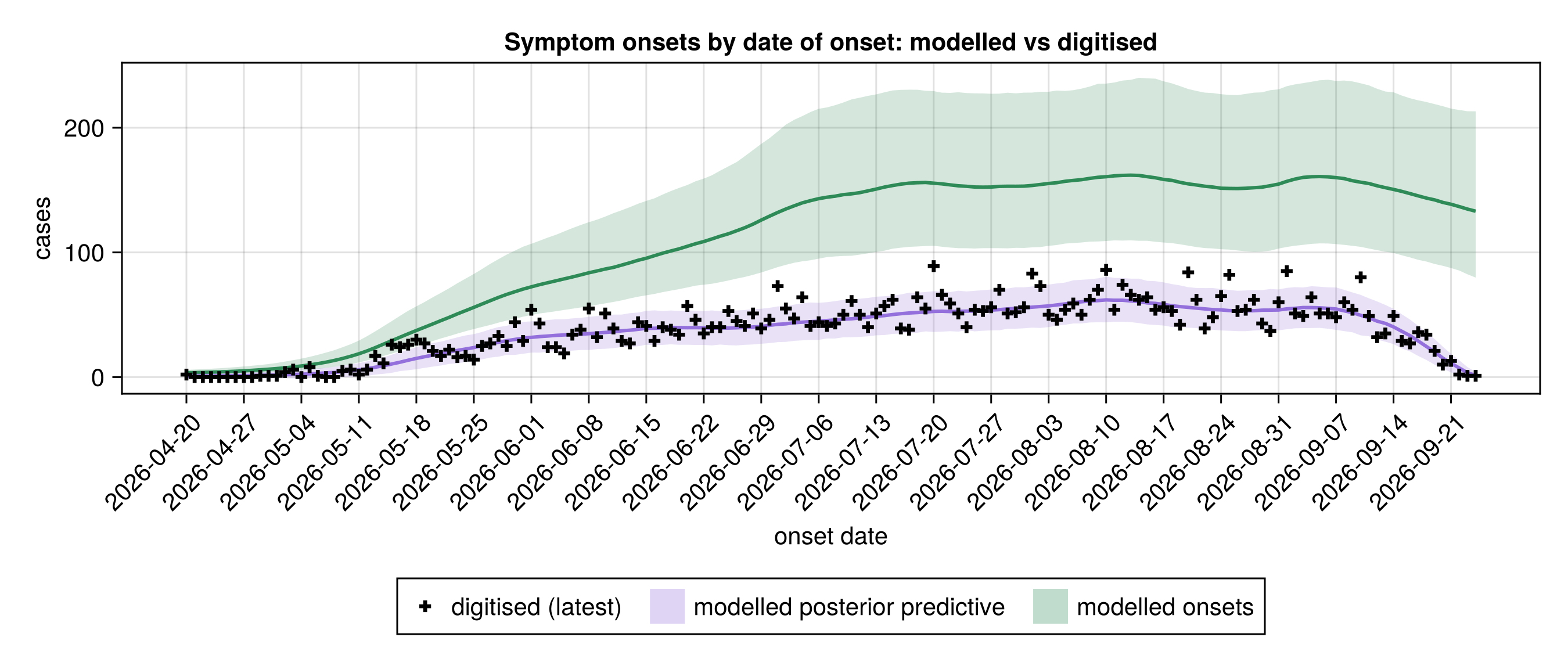
Counterfactual: lower bound under no further transmission
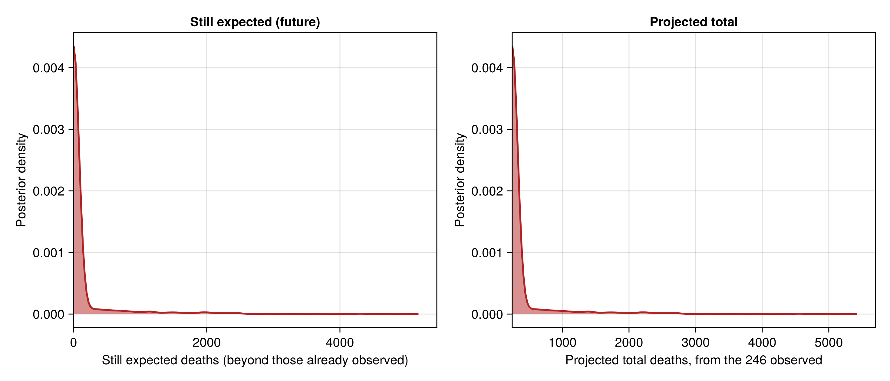
is the committed future deaths if transmission stopped at the report date, defined in the no-onward-transmission counterfactual Methods section.
Project no-onward deaths and summarise
no_onward = predict_no_onward_deaths(
    chn_joint; obs_deaths = obs.total_deaths
);

no_onward_table = streams_table(
    "no-onward total" => no_onward.total_projected;
    digits = 0
);| Row | Stream | Lower 90% | Lower 60% | Lower 30% | Upper 30% | Upper 60% | Upper 90% |
|---|---|---|---|---|---|---|---|
| String | Float64 | Float64 | Float64 | Float64 | Float64 | Float64 | |
| 1 | no-onward total | 246.0 | 246.0 | 246.0 | 246.0 | 246.0 | 999.0 |
The left panel shows the still expected deaths
No-onward projected-deaths plot
no_onward_fig = plot_no_onward_deaths(
    no_onward; obs_deaths = obs.total_deaths
);
Confirmed case-fatality ratio
The delay-corrected confirmed CFR, defined in the delay-corrected confirmed CFR Methods section, is set against the structural (infection-based) CFR and the naive confirmed ratio. The corrected ratio debiases the naive confirmed ratio for the real-time delay between a case being confirmed and a death being confirmed. The structural CFR is the onset-level estimate the joint model fits.
Compute the confirmed-CFR comparison
confirmed_cfr = delay_corrected_confirmed_cfr(
    chn_joint;
    obs_confirmed = obs.confirmed_cases,
    obs_confirmed_deaths = obs.confirmed_deaths
);

confirmed_cfr_summary = confirmed_cfr_table(confirmed_cfr);

# Summary line carrying the data-anchored corrected estimate alongside the
# infection-based structural CFR, so both can be quoted together.
confirmed_cfr_line = let r = confirmed_cfr
    pct(x) = round(100 * x; digits = 1)
    corr = filter(isfinite, r.corrected)
    struc = filter(isfinite, r.structural)
    cs = posterior_summary(corr)
    ss = posterior_summary(struc)
    Markdown.parse(
        string(
            "**Delay-corrected confirmed CFR:** ",
            pct(quantile(corr, 0.5)), "% (90% CrI ",
            pct(cs.lo90), "–", pct(cs.hi90), "%), versus a naive confirmed ratio ",
            "of ", pct(r.naive_observed), "% and a structural (infection-based) ",
            "CFR of ", pct(quantile(struc, 0.5)), "% (90% CrI ",
            pct(ss.lo90), "–", pct(ss.hi90), "%)."
        )
    )
end;
Delay-corrected confirmed CFR: 47.1% (90% CrI 42.6–51.6%), versus a naive confirmed ratio of 48.4% and a structural (infection-based) CFR of 47.1% (90% CrI 36.8–58.4%).
| Row | Quantity | Estimate |
|---|---|---|
| String | String | |
| 1 | Delay-corrected confirmed CFR | 42.6–51.6% |
| 2 | Structural (infection-based) CFR | 36.8–58.4% |
| 3 | Uncorrected modelled confirmed ratio | 38.6–46.0% |
| 4 | Naive observed confirmed ratio | 48.4% |
The figure below shows the posterior densities of the delay-corrected confirmed CFR and the structural CFR. The naive observed confirmed ratio is drawn as a solid vertical rule, and the median uncorrected modelled confirmed ratio as a dashed rule. The gap from the naive rule to the corrected density is the real-time delay debiasing. The gap to the structural density is the residual case/death ascertainment difference.
Confirmed-CFR density plot
confirmed_cfr_fig = plot_confirmed_cfr(confirmed_cfr);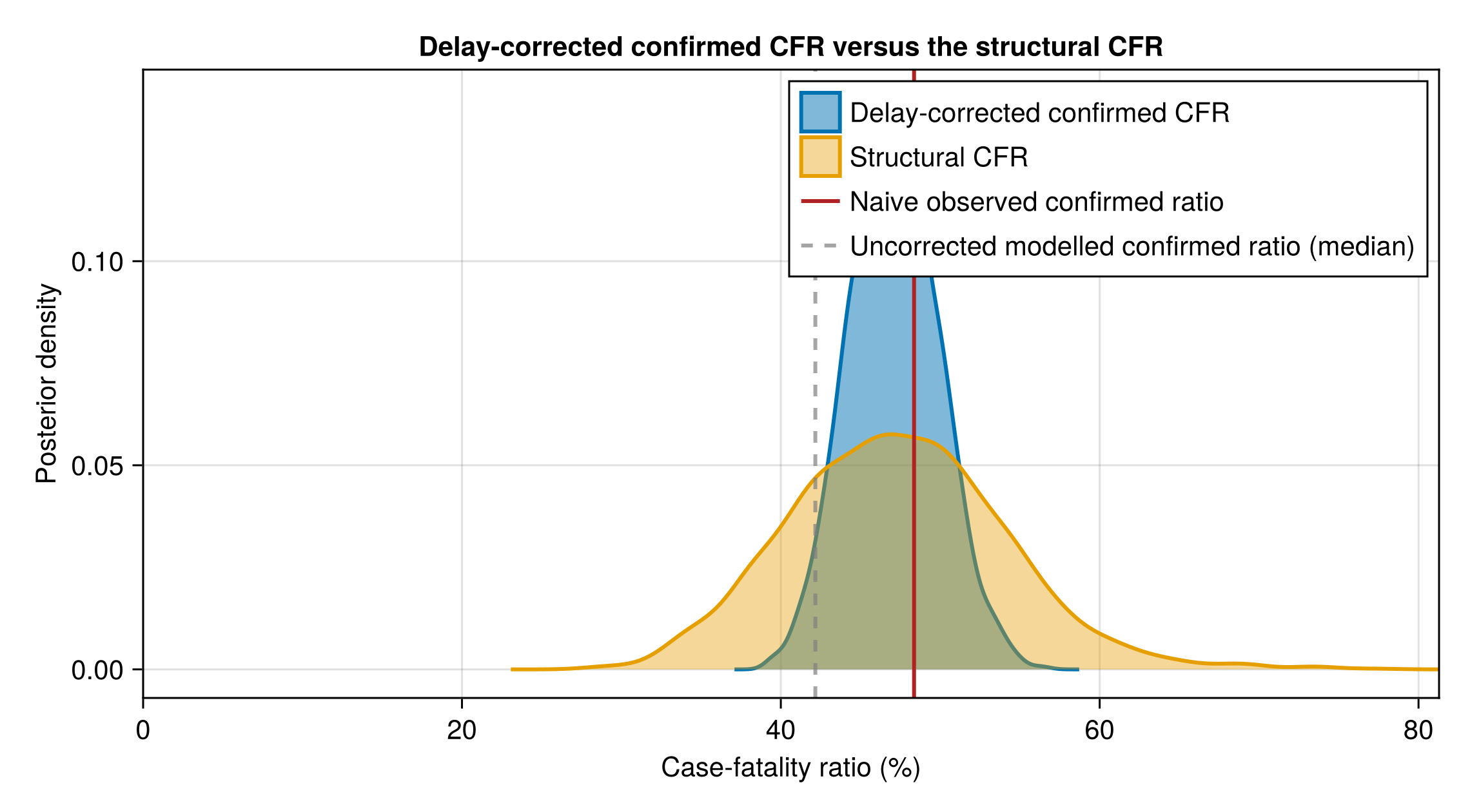
The same ratios by province are in the case-fatality ratio by province.
Forecast results
The one-week-ahead projection of every stream, the symptom-onset nowcast and the scoring against what arrived are on the forecasts page.
Saving results
The tables above are written to an output directory at the repo root so they can be archived and shared. On every push to the main branch a GitHub Actions workflow regenerates these files and publishes them as a GitHub Release, downloadable from the repository's releases page (https://github.com/epiforecasts/BVDOutbreakSize/releases). The release bundles the summary tables, a thinned set of posterior draws, the latent symptom-onset ("symptomatic cases") trajectory over time, the one- to four-week-ahead forecasts of the observed streams, and a copy of the input data manifest.
Write outputs to output/
# Outputs default to `output/` in the package directory (where the
# docs build and Release workflow expect them). Set `BVD_OUTPUT_DIR`
# to redirect them, e.g. when running from a read-only package
# install.
output_dir = get(
    ENV, "BVD_OUTPUT_DIR",
    joinpath(pkgdir(BVDOutbreakSize), "output")
)
mkpath(output_dir)

# Full parameter summary for the published CSV (infection, surveillance and
# export parameters together).
joint_summary = summary_table(
    chn_joint,
    [
        :r, :r0, :doubling_time, :T, :R_T, :CFR, :C_T,
        :p_drc, :p_uganda, :k, :tau_test, :lambda_bg,
        Symbol("exports_state.travel_state.daily_travellers"),
    ]; digits = 2
)
CSV.write(joinpath(output_dir, "posterior_summary.csv"), joint_summary)
CSV.write(
    joinpath(output_dir, "confirmed_cfr_summary.csv"),
    confirmed_cfr_summary
)

# Copy the input data so the release records what produced these
# results.
cp(
    joinpath(pkgdir(BVDOutbreakSize), "data", "observations.toml"),
    joinpath(output_dir, "observations.toml"); force = true
)

# Thinned posterior draws of the key joint parameters (every 10th
# draw) so downstream users can recompute their own summaries.
# `cumulative_onsets_T` is the cumulative symptom onsets by the cut-off,
# the latent "symptomatic cases" outcome (the onset analogue of `C_T`),
# read off the last day of each draw's `cumulative_onsets` trajectory.
_cum_onset_draws = vec(collect(chn_joint[:cumulative_onsets]))
cumulative_onsets_T = Float64[v[end] for v in _cum_onset_draws]
# Raw walk base `log_R0`, the renewal reproduction-number walk's starting
# point on the log scale, kept unexponentiated so downstream scoring takes
# its own exp. This is a distinct quantity from `r0`, the growth-clock
# initial rate, so both columns are published side by side.
log_R0_draws = vec(Array(chn_joint[Symbol("rt_state.log_R0")]))
posterior_draws = DataFrame(
    r = vec(Array(chn_joint[:r])),
    r0 = vec(Array(chn_joint[:r0])),
    doubling_time = vec(Array(chn_joint[:doubling_time])),
    T = vec(Array(chn_joint[:T])),
    R_T = vec(Array(chn_joint[:R_T])),
    CFR = vec(Array(chn_joint[:CFR])),
    p_drc = vec(Array(chn_joint[:p_drc])),
    p_uganda = vec(Array(chn_joint[:p_uganda])),
    C_T = vec(Array(chn_joint[:C_T])),
    cumulative_onsets_T = cumulative_onsets_T,
    confirmed_cfr_corrected = confirmed_cfr.corrected
)
posterior_draws[!, Symbol("rt_state.log_R0")] = log_R0_draws
posterior_draws = posterior_draws[1:10:end, :]
CSV.write(joinpath(output_dir, "posterior_draws.csv"), posterior_draws);

# One- to four-week-ahead forecasts of the observed streams, saved as a
# release asset so each release records the forecast it made and it can later
# be scored against what is observed. Only the incident and level quantities
# are archived (see `forecast_archive`), thinned to keep the asset compact.
forecast_horizons = (7, 14, 21, 28)
forecast_joint_draws = fit_forecast("joint")
forecast_runs = [
    (
        h,
        forecast_reported(
            forecast_joint_draws; horizon = h,
            obs_cases = obs.reported_cases,
            obs_deaths = obs.total_deaths,
            obs_confirmed = obs.confirmed_cases,
            obs_confirmed_deaths = obs.confirmed_deaths,
            obs_recovered = obs.recovered_cases
        ),
    )
        for h in forecast_horizons
]
CSV.write(
    joinpath(output_dir, "forecast.csv"),
    forecast_archive(forecast_runs; made_date = obs.cutoff, thin = 5)
);

# The province forecast archive, in the `forecast.csv` schema plus the
# province each row belongs to, so a release records the provincial forecast
# it made alongside the national one.
CSV.write(
    joinpath(output_dir, "province_forecast.csv"),
    province_forecast_archive(
        forecast_joint_draws, forecast_runs;
        made_date = obs.cutoff, n_patches = N_PATCHES, thin = 5
    )
);

# The same one- to four-week-ahead forecast made from each FROZEN joint
# re-fit (the McCabe-matched cut-offs, the Chamla anchor and the one-week-back
# validation fit), each stamped with its OWN cut-off as the made date. This
# gives historical forecast evaluation using the current model at past data
# cut-offs, scored against what has since been observed, without
# reconstructing old release tags. Each frozen fit uses its own frozen
# observations for the cut-off counts. The May cut-offs predate the isolation
# and recovered streams, so those are simply absent for them; the per-stream
# guard in `forecast_archive` skips a stream a fit does not carry.
frozen_forecast_ids = unique(
    id -> load_fit(id).o.cutoff,
    [
        ["frozen_$c" for c in frozen_cutoffs];
        "frozen_$chamla_cutoff"; "frozen_validation"
    ]
)
# The `fit` column tells the frozen joint and each frozen single-stream fit
# apart when scored. `score_release` falls back to one default where an
# archive carries no such column, so an older release still scores as the
# joint.
frozen_forecast_archive = DataFrame(
    made_date = Date[], horizon = Int[],
    target_date = Date[], stream = String[], draw = Int[], value = Float64[],
    fit = String[]
)
# Each frozen model is rebuilt from its own frozen observations, so the May
# cut-offs, which predate the digitised onset figure, carry no onset
# forecast.
for id in frozen_forecast_ids
    _fo = load_fit(id).o
    _fpp = fit_forecast(id)
    runs = [
        (
            h,
            forecast_reported(
                _fpp; horizon = h,
                obs_cases = _fo.reported_cases,
                obs_deaths = _fo.total_deaths,
                obs_confirmed = _fo.confirmed_cases,
                obs_confirmed_deaths = _fo.confirmed_deaths,
                obs_recovered = _fo.recovered_cases
            ),
        )
            for h in forecast_horizons
    ]
    _rows = forecast_archive(runs; made_date = _fo.cutoff, thin = 5)
    _rows[!, :fit] = fill(FROZEN_FIT, size(_rows, 1))
    append!(frozen_forecast_archive, _rows)
end

# The frozen single-stream fits, forecast from their own chains as
# `stream_forecasts.csv` forecasts the live ones. They are registered only
# at the validation cut-off and only for still-reported streams.
_frozen_stream_of = Dict(
    "cases" => (:reported_cases, "reported cases"),
    "deaths" => (:suspected_deaths, "suspected deaths"),
    "confirmed" => (:confirmed_cases, "confirmed cases"),
    "confirmed_deaths" => (:confirmed_deaths, "confirmed deaths"),
    "treatment" => (:isolation_beds, "isolation beds")
)
for (_sid, _sf) in sort(collect(pairs(frozen_lastweek_streams)); by = first)
    _stream, _label = _frozen_stream_of[_sid]
    _o = _sf.o
    _spp = fit_forecast("frozen_validation_$_sid")
    for h in forecast_horizons
        _vals = forecast_stream(_spp, _stream; horizon = h)
        for (_d, _i) in enumerate(1:5:length(_vals))
            push!(
                frozen_forecast_archive,
                (
                    _o.cutoff, h, _o.cutoff + Day(h), _label, _d,
                    Float64(_vals[_i]), _sid,
                )
            )
        end
    end
end
CSV.write(
    joinpath(output_dir, "forecast_frozen.csv"),
    frozen_forecast_archive
);

# Per-fit release assets: the reproduction number, outbreak size and forecasts
# for every fit rather than the joint alone, so a release records what each
# dataset implies on its own and can later be scored against the joint. The
# single-stream fits walk Rt from day 1 while the joint walks from
# `RT_WALK_LEAD` days before the first situation report, so each fit carries
# the starts its own fit used. Each single-stream fit forecasts only the
# dataset it observes; the joint forecasts every shared stream. Recovered has
# no single-stream fit, so the joint is the only fit that carries it.
stream_thin = 5
_rt_walk_start_joint = clamp(_BREAKPOINT - RT_WALK_LEAD, _rt_start_plot, obs.n)
stream_fits = [
    (;
        fit = "joint", chn = chn_joint, rt_start = _rt_start_plot,
        rt_walk_start = _rt_walk_start_joint,
        streams = [
            (:reported_cases, "reported cases"),
            (:suspected_deaths, "suspected deaths"),
            (:confirmed_cases, "confirmed cases"),
            (:confirmed_deaths, "confirmed deaths"),
            (:recovered, "recovered"),
            (:isolation_beds, "isolation beds"),
            (:exports, "exports"),
            (:onset_reports, "onset reports"),
        ],
    ),
    (;
        fit = "cases", chn = chn_cases, rt_start = 1, rt_walk_start = 1,
        streams = [(:reported_cases, "reported cases")],
    ),
    (;
        fit = "deaths", chn = chn_deaths, rt_start = 1, rt_walk_start = 1,
        streams = [(:suspected_deaths, "suspected deaths")],
    ),
    (;
        fit = "confirmed", chn = chn_confirmed, rt_start = 1, rt_walk_start = 1,
        streams = [(:confirmed_cases, "confirmed cases")],
    ),
    (;
        fit = "confirmed_deaths", chn = chn_confirmed_deaths, rt_start = 1,
        rt_walk_start = 1,
        streams = [
            (:confirmed_deaths, "confirmed deaths"),
        ],
    ),
    (;
        fit = "treatment", chn = chn_treatment, rt_start = 1,
        rt_walk_start = 1,
        streams = [(:isolation_beds, "isolation beds")],
    ),
    (;
        fit = "exports", chn = chn_exports, rt_start = 1, rt_walk_start = 1,
        streams = [(:exports, "exports")],
    ),
    (;
        fit = "onsets", chn = chn_onsets, rt_start = 1, rt_walk_start = 1,
        streams = [(:onset_reports, "onset reports")],
    ),
]

# Cut-off reproduction number per fit. The joint exposes it as `R_T`; the
# single-stream composers do not (the alias lives in `bvd_joint`, not the
# shared latent submodel), so theirs is rebuilt from the walk parameters every
# chain carries and read at the cut-off, the last day of the reconstructed
# path. `ramp` matches the model's 21-day intervention scale-up.
function _fit_rt_draws(f)
    f.fit == "joint" && return vec(Array(f.chn[:R_T]))
    rt = reconstruct_rt(
        f.chn; n = obs.n, breakpoint = _BREAKPOINT,
        rt_start = f.rt_start, rt_walk_start = f.rt_walk_start, ramp = RT_INTERVENTION_RAMP
    )
    return Float64[rt[i, obs.n] for i in axes(rt, 1)]
end

# Basic reproduction number per fit, the renewal walk's starting value, a
# single distribution per fit rather than a daily series. Every current
# single-stream composer shares the joint's latent submodel and so carries
# its own walk base, but `r0_walk_draws` probes rather than assumes, so a
# single-stream model built without its own renewal walk drops out of this
# quantity instead of breaking the release.
_stream_quantities = [
    (
        f.fit, _fit_rt_draws(f), vec(Array(f.chn[:C_T])),
        r0_walk_draws(f.chn),
    ) for f in stream_fits
]

# One row per fit and quantity, with the median and the 30/60/90% credible
# bounds the report's tables use.
function _stream_estimate_row(fit, quantity, draws)
    s = posterior_summary(draws)
    return (
        fit = fit, quantity = quantity, median = quantile(draws, 0.5),
        lo30 = s.lo30, hi30 = s.hi30, lo60 = s.lo60, hi60 = s.hi60,
        lo90 = s.lo90, hi90 = s.hi90,
    )
end
stream_estimates = DataFrame(
    [
        _stream_estimate_row(fit, q, d)
            for (fit, rt, ct, r0) in _stream_quantities
            for (q, d) in (
                ("R_T", rt), ("C_T", ct),
                ("R0", r0),
            )
            if !isnothing(d)
    ]
)
CSV.write(joinpath(output_dir, "stream_estimates.csv"), stream_estimates);

# Thinned reproduction-number and outbreak-size draws per fit, so downstream
# scoring can recompute its own summaries rather than reuse the intervals.
stream_draws = DataFrame(
    [
        (fit = fit, quantity = q, draw = d, value = v)
            for (fit, rt, ct, r0) in _stream_quantities
            for (q, vals) in (
                ("R_T", rt), ("C_T", ct),
                ("R0", r0),
            )
            if !isnothing(vals)
            for (d, v) in enumerate(vals[1:stream_thin:end])
    ]
)
CSV.write(joinpath(output_dir, "stream_draws.csv"), stream_draws);

# Per-fit forecasts of each fit's own observed stream, in the `forecast.csv`
# long schema plus the fit that made them, each drawn from that fit's own
# model run past the cut-off.
stream_forecasts = DataFrame(
    made_date = Date[], horizon = Int[],
    target_date = Date[], stream = String[], draw = Int[], value = Float64[],
    fit = String[]
)
for f in stream_fits, (stream, label) in f.streams,
        h in forecast_horizons
    _vals = forecast_stream(fit_forecast(f.fit), stream; horizon = h)
    for (d, i) in enumerate(1:stream_thin:length(_vals))
        push!(
            stream_forecasts, (
                obs.cutoff, h, obs.cutoff + Day(h), label,
                d, Float64(_vals[i]), f.fit,
            )
        )
    end
end

# Confirmed/suspect ward-bed occupancy for the joint, read from the joint's
# own `forecast_reported` runs so the ward beds are scored on the same
# footing as the total occupancy in the preferred `stream_forecasts.csv`
# asset. `forecast_stream` cannot project these. The split is not a growable
# stream but a partition of the total.
#
# Dead as it stands. `forecast_reported` projects the total occupancy alone
# and emits neither column, so the guard below always skips and nothing
# reaches `stream_forecasts.csv` under these two labels. The joint does
# carry the cut-off split (`expected_confirmed_incare_T`), so what is
# missing is the partition of the projected level, not the quantity to
# partition it by. Kept, with the guard, so the loop starts writing the
# moment `forecast_reported` grows those columns.
for (h, fc) in forecast_runs,
        (col, label) in (
            (:suspect_occupancy, "isolation beds (suspected)"),
            (:confirmed_occupancy, "treatment beds"),
        )

    col in propertynames(fc) || continue
    _wvals = fc[!, col]
    for (d, i) in enumerate(1:stream_thin:length(_wvals))
        push!(
            stream_forecasts, (
                obs.cutoff, h, obs.cutoff + Day(h), label,
                d, Float64(_wvals[i]), "joint",
            )
        )
    end
end
CSV.write(joinpath(output_dir, "stream_forecasts.csv"), stream_forecasts);

# Latent symptom-onset trajectory over time, the "symptomatic cases" curve,
# showing outbreak growth: one row per grid day with the 30/60/90%
# credible intervals of both the daily new and cumulative onsets.
onsets_over_time_table = onsets_over_time(
    chn_joint;
    n = obs.n, seeding = obs.seeding
)
CSV.write(
    joinpath(output_dir, "onsets_over_time.csv"),
    onsets_over_time_table
);
Summary-page assets
The one-page Summary dashboard reuses the results computed above rather than re-fitting. Here we save its headline text, headline tables and the figures it shows (the national reproduction number and infections over time) into docs/src/summary_assets/. The static dashboard page embeds them after this build step has run.
Write the dashboard assets
dashboard_dir = joinpath(
    pkgdir(BVDOutbreakSize), "docs", "src", "summary_assets"
)
mkpath(dashboard_dir)

# Figures: estimated R(t) nationally and latent infections over time, both
# produced in the Results sections above and written here at the dashboard
# size. The province and in-sample pages write the figures they own.
CairoMakie.save(joinpath(dashboard_dir, "rt.png"), rt_fig)
CairoMakie.save(
    joinpath(dashboard_dir, "infections.png"),
    cumulative_traj_fig
)

# Headline prose: the same bullet summary shown at the top of the Results
# section, serialised to markdown so the dashboard renders it verbatim.
open(joinpath(dashboard_dir, "headline.md"), "w") do io
    print(io, sprint(Markdown.plain, summary_ranges))
end

# Headline tables: outbreak size and timing as whole numbers, and the
# growth and severity parameters to two decimals, each with reader-friendly
# quantity names.
dashboard_counts = summary_table(
    chn_joint, [:C_T, :T]; digits = 0,
    labels = Dict(
        :C_T => "Cumulative infections",
        :T => "Outbreak age (days)"
    )
)
dashboard_rates = summary_table(
    chn_joint,
    [:R0, :R_T, :r, :doubling_time, :CFR]; digits = 2,
    labels = Dict(
        :R0 => "Initial reproduction number",
        :R_T => "Latest reproduction number",
        :r => "Latest growth rate (per day)",
        :doubling_time => "Latest doubling time (days)",
        :CFR => "Case-fatality ratio"
    )
)
open(joinpath(dashboard_dir, "headline_counts.md"), "w") do io
    print(io, markdown_table(dashboard_counts))
end
open(joinpath(dashboard_dir, "headline_rates.md"), "w") do io
    print(io, markdown_table(dashboard_rates))
end

# Fit diagnostics: the same summary and table the Results section shows,
# so the dashboard reports how the fit behind its numbers sampled without
# building a second table.
open(joinpath(dashboard_dir, "diagnostics.md"), "w") do io
    print(io, fit_diagnostics_detail_md, "\n\n")
    print(io, markdown_table(fit_diagnostics_table))
end
open(joinpath(dashboard_dir, "diagnostics_summary.md"), "w") do io
    print(io, fit_convergence_summary.verdict)
end

# The data cut-off the dashboard reports as of, written as a plain date.
open(joinpath(dashboard_dir, "cutoff.md"), "w") do io
    print(io, string(obs.cutoff))
end
The full analysis code, data and model definitions are in the epiforecasts/BVDOutbreakSize repository. Issues, corrections and suggestions are welcome there. Maintained by Sam Abbott, Kath Sherratt, Samuel Brand and Sebastian Funk.