Province estimates

This page gives the province estimates from the joint model. The methods for this model are on the Methods page.

The model runs one renewal equation per province and fits the national streams against the summed provinces, so the national estimates are the sum of the provinces here. The per-province forecast is on the province forecasts page and its scoring is in the forecast by province.

This page is generated from docs/pages/estimates/province.jl. The model code it calls is in src/. See aim and origins and limitations.

Load packages, data and fitted chains

# Shared setup: packages, observations and the fit registry. See
# `docs/pages/_setup.jl`.
using BVDOutbreakSize
include(joinpath(pkgdir(BVDOutbreakSize), "docs", "pages", "_setup.jl"))

validation_forecast_from (generic function with 1 method)

# The fits this page reads, loaded from the cache here.
chn_joint = load_fit("joint");

Last updated: 30 September 2026.

Data as of: 26 September 2026.

Summary

The table below compares the provinces, from the joint posterior. Each range is an equal-tailed 90% credible interval, and the shares and probabilities are computed draw by draw. The reproduction number and the relative case ascertainment are identified only as a product, and the per-province deaths break the tie.

Compute the province comparison

province_headline_md = patch_headline(chn_joint, N_PATCHES)
province_headline = Markdown.parse(province_headline_md);

Province	Share of infections (%)	R at the cut-off	P(R > 1)	CFR (%)	Relative ascertainment
Ituri	65–75	0.55–1.26	26%	34.4–59.9	0.92–1.31
Nord-Kivu	20–29	0.48–1.31	26%	37.5–67.2	0.73–1.07
Haut-Uele	3–6	0.51–1.57	37%	34.6–58.8	0.89–1.25
Other provinces	1–1	0.66–1.96	67%	34.4–59.8	0.79–1.2

Ituri has the most infections with probability over 99%, and 1 of 4 provinces is more likely than not to be growing. Infections imported from another province make up 0.0–0.4% of infections to date.

Maps

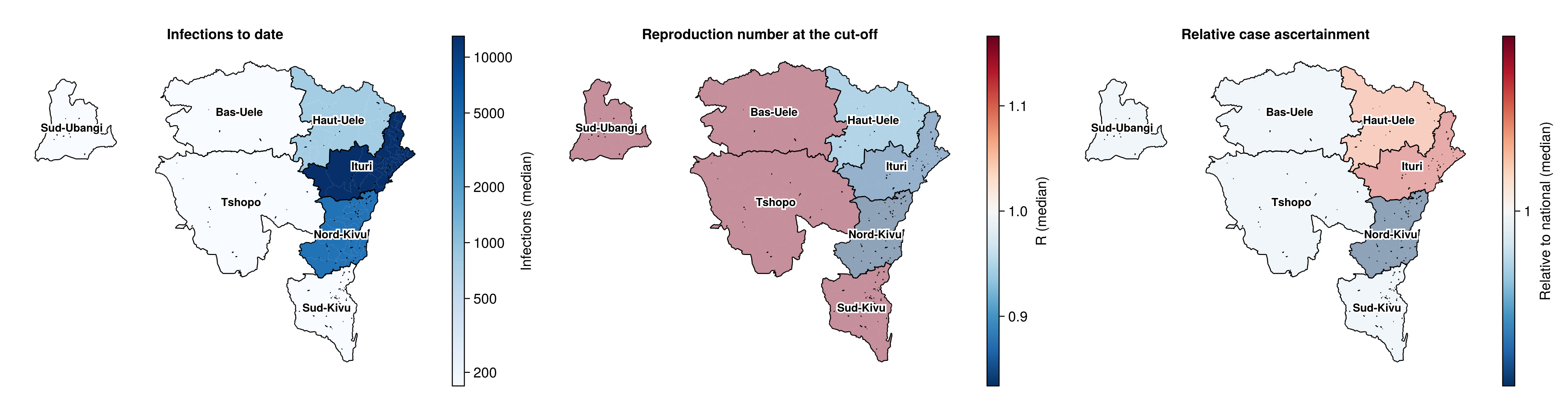
The maps shade each province by its patch's posterior median, so the pooled patch shades all its provinces alike. The reproduction number at the cut-off and the relative case ascertainment are centred on one, and a province whose 90% credible interval spans one is washed out. The Methods page defines each quantity.

Maps of infections, reproduction number and ascertainment

province_map_fig = plot_province_map(
    [
        (;
            values = province_map_summary(
                chn_joint, :C_T_patch, N_PATCHES
            ).values,
            title = "Infections to date", scale = log10,
            colorbar_label = "Infections (median)",
        ),
        (;
            province_map_summary(chn_joint, :R_T_patch, N_PATCHES)...,
            title = "Reproduction number at the cut-off",
            diverging_at = 1.0, colorbar_label = "R (median)",
        ),
        (;
            province_map_summary(
                chn_joint, :province_ascertainment, N_PATCHES
            )...,
            title = "Relative case ascertainment", diverging_at = 1.0,
            scale = log10, colorbar_label = "Relative to national (median)",
        ),
    ]
);

Detail by province

Each province's own estimates are below, as equal-tailed 30%, 60% and 90% credible intervals, with its case-fatality ratio in the case-fatality ratio by province. The log-Rt deviation is from the national trend, the drift is the deviation's walk scale and the contrast is against Ituri.

Compute the per-province tables and figure

# The tables below and the pair-plot dropdowns further down name the
# provinces in this order.
@assert PROVINCE_LABELS[1:N_PATCHES] ==
    ["Ituri", "Nord-Kivu", "Haut-Uele", "Other provinces"]
province_detail_tables = [
    patch_summary_table(chn_joint, N_PATCHES; patch = p) for p in 1:N_PATCHES
];
province_detail_fig = plot_patch_summary(chn_joint, N_PATCHES);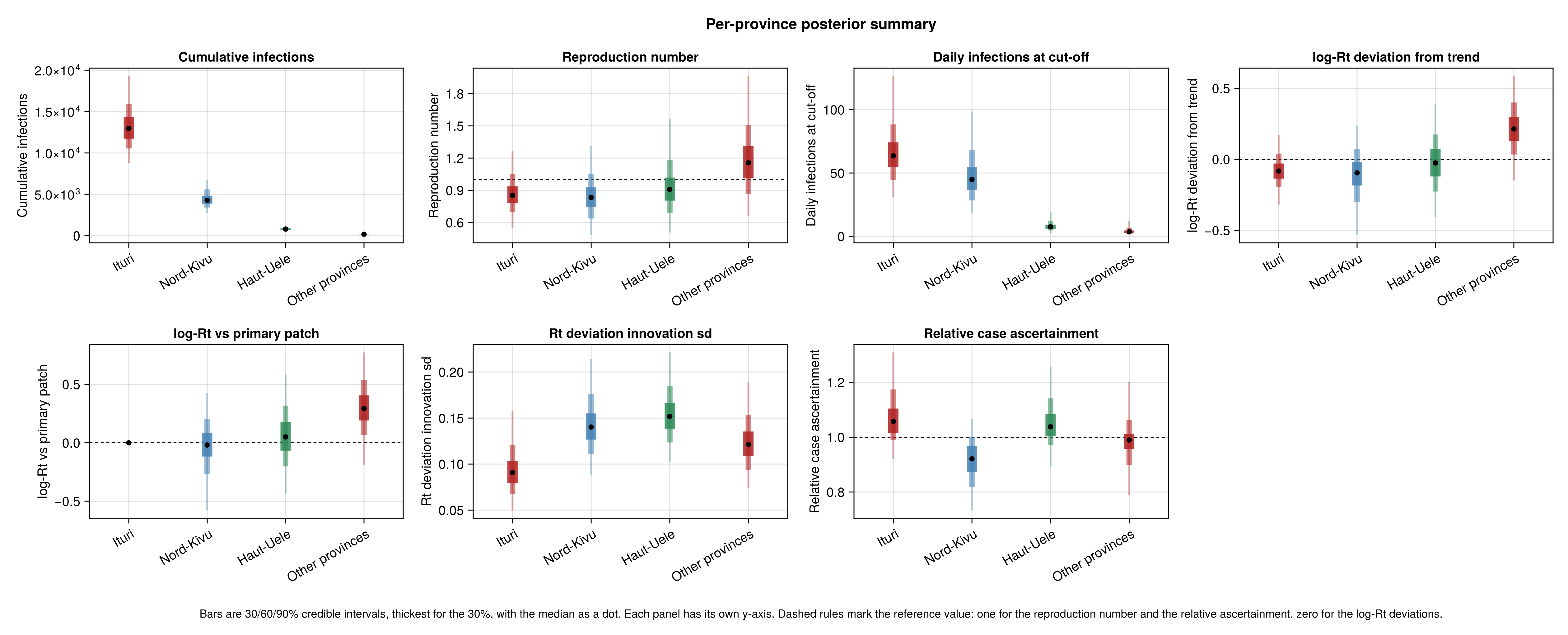

Ituri

7×7 DataFrame

Row	Quantity	Lower 90%	Lower 60%	Lower 30%	Upper 30%	Upper 60%	Upper 90%
	String	Float64	Float64	Float64	Float64	Float64	Float64
1	Cumulative infections	8736.0	10542.0	11716.0	14297.0	15933.0	19280.0
2	Reproduction number	0.55	0.69	0.78	0.94	1.05	1.26
3	Daily infections at cut-off	31.0	44.0	55.0	74.0	88.0	127.0
4	log-Rt deviation from trend	-0.32	-0.2	-0.14	-0.03	0.04	0.17
5	log-Rt vs primary patch	0.0	0.0	0.0	0.0	0.0	0.0
6	Rt deviation innovation sd	0.05	0.067	0.079	0.104	0.121	0.158
7	Relative case ascertainment	0.92	0.99	1.02	1.1	1.17	1.31

Nord-Kivu

7×7 DataFrame

Row	Quantity	Lower 90%	Lower 60%	Lower 30%	Upper 30%	Upper 60%	Upper 90%
	String	Float64	Float64	Float64	Float64	Float64	Float64
1	Cumulative infections	2758.0	3401.0	3856.0	4811.0	5592.0	6771.0
2	Reproduction number	0.48	0.64	0.74	0.93	1.06	1.31
3	Daily infections at cut-off	18.0	28.0	37.0	55.0	68.0	99.0
4	log-Rt deviation from trend	-0.53	-0.3	-0.18	-0.02	0.07	0.24
5	log-Rt vs primary patch	-0.58	-0.27	-0.12	0.09	0.2	0.42
6	Rt deviation innovation sd	0.088	0.111	0.127	0.155	0.176	0.214
7	Relative case ascertainment	0.73	0.82	0.87	0.97	1.0	1.07

Haut-Uele

7×7 DataFrame

Row	Quantity	Lower 90%	Lower 60%	Lower 30%	Upper 30%	Upper 60%	Upper 90%
	String	Float64	Float64	Float64	Float64	Float64	Float64
1	Cumulative infections	514.0	630.0	715.0	898.0	1031.0	1283.0
2	Reproduction number	0.51	0.69	0.8	1.02	1.18	1.57
3	Daily infections at cut-off	3.0	5.0	6.0	9.0	12.0	20.0
4	log-Rt deviation from trend	-0.41	-0.23	-0.12	0.07	0.17	0.39
5	log-Rt vs primary patch	-0.44	-0.2	-0.07	0.18	0.32	0.59
6	Rt deviation innovation sd	0.103	0.123	0.139	0.166	0.185	0.221
7	Relative case ascertainment	0.89	0.97	1.0	1.08	1.14	1.25

Other provinces

7×7 DataFrame

Row	Quantity	Lower 90%	Lower 60%	Lower 30%	Upper 30%	Upper 60%	Upper 90%
	String	Float64	Float64	Float64	Float64	Float64	Float64
1	Cumulative infections	98.0	129.0	148.0	192.0	227.0	306.0
2	Reproduction number	0.66	0.86	1.02	1.31	1.51	1.96
3	Daily infections at cut-off	1.0	2.0	3.0	5.0	7.0	12.0
4	log-Rt deviation from trend	-0.15	0.03	0.13	0.3	0.4	0.59
5	log-Rt vs primary patch	-0.19	0.07	0.19	0.41	0.54	0.77
6	Rt deviation innovation sd	0.074	0.093	0.109	0.135	0.154	0.189
7	Relative case ascertainment	0.79	0.9	0.96	1.01	1.06	1.2

Isolation beds

Beds, bed demand, occupied beds, utilisation and demand above the beds by province at the cut-off, from the per-province occupancy and bed figures the situation reports print. Each province's beds are its modelled capacity floored at its last recorded effective beds, which cover the patients each report counts. Its occupied beds are its demand share of the national modelled occupancy, capped at its beds, and the rest is the demand above the beds. The provinces sum to the national figures, and no province's utilisation exceeds 100%.

Province bed table

province_bed_overview = province_bed_table(chn_joint, N_PATCHES);

4×6 DataFrame

Row	Province	Beds	Bed demand	Occupied beds	Utilisation (%)	Demand above beds
	String	String	String	String	String	String
1	Ituri	1015 (1015–1059)	511 (456–566)	453 (413–492)	44.3 (40.4–48.2)	0 (0–0)
2	Nord-Kivu	354 (354–354)	318 (282–355)	281 (254–310)	79.5 (71.8–87.7)	0 (0–0)
3	Haut-Uele	138 (138–144)	58 (49–68)	51 (43–60)	36.8 (31.3–43.0)	0 (0–0)
4	Other provinces	28 (28–28)	37 (30–45)	28 (26–28)	100.0 (94.0–100.0)	5 (0–12)

Size and infections

The national outbreak size in the joint model estimates is the sum of the four patches' renewal equations. The figure below shows the modelled infections behind those totals, daily on the top row and cumulative on the bottom.

Modelled infections by province

province_infections_fig = plot_infections_patches(
    chn_joint;
    n = obs.n, seeding = obs.seeding, n_patches = N_PATCHES
);

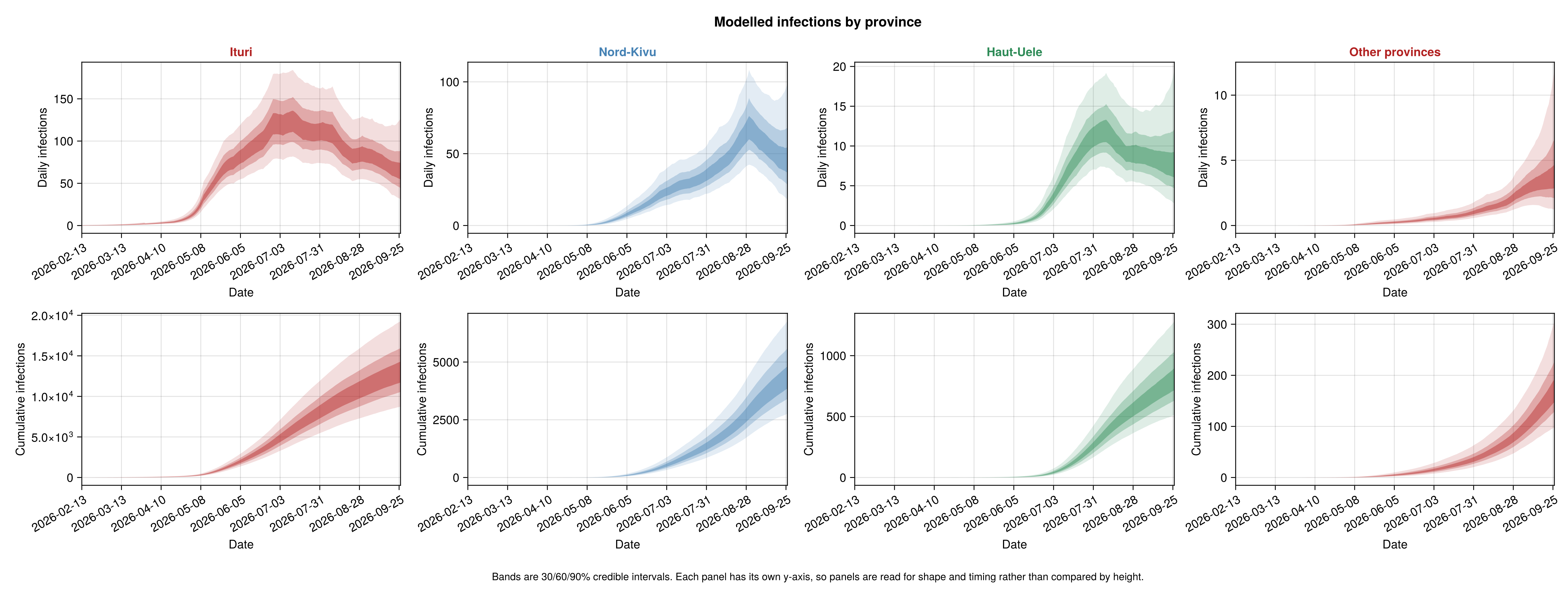
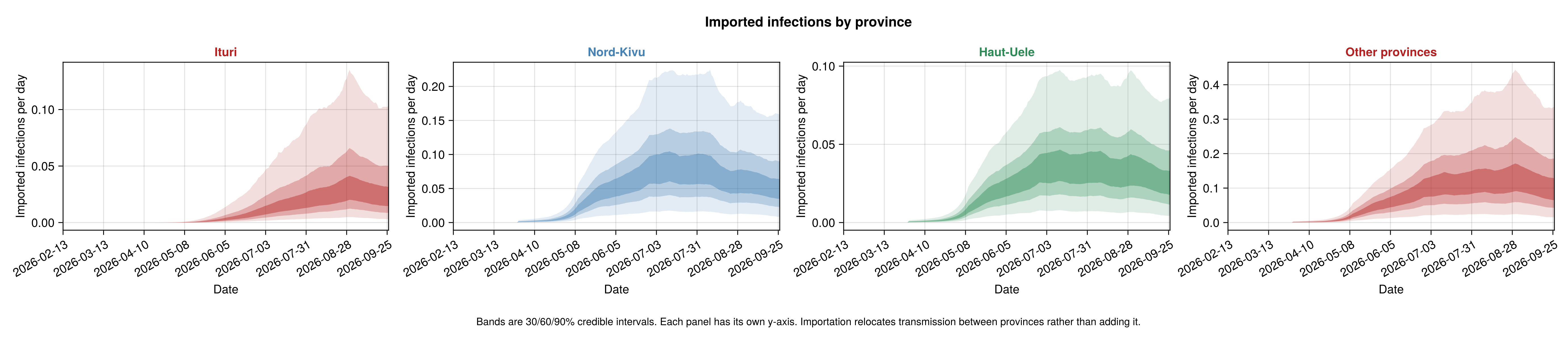
The provinces are coupled by a gravity kernel weighted by destination population, described in the mixing and importation Methods section, with its intensity estimated. Every arrival is debited from its origin the same day, so the figure reads as where infection occurred rather than as extra infection. The distances between the patches' population centres are 324 km from Ituri to Nord-Kivu, 216 km from Ituri to Haut-Uele and 390 km from Nord-Kivu to the pooled patch, so most of what leaves Nord-Kivu lands in the pooled patch.

Importation intensity and imports by province

importation_table = summary_table(
    chn_joint, [:importation_epsilon];
    digits = 4,
    labels = Dict(:importation_epsilon => "Importation intensity")
);

province_imports_fig = plot_imports_patches(
    chn_joint;
    n = obs.n, seeding = obs.seeding, n_patches = N_PATCHES
);

1×7 DataFrame

Row	Quantity	Lower 90%	Lower 60%	Lower 30%	Upper 30%	Upper 60%	Upper 90%
	String	Float64	Float64	Float64	Float64	Float64	Float64
1	Importation intensity	0.0005	0.0011	0.0016	0.0027	0.0037	0.0066

Reproduction number by province

The national reproduction number is in reproduction number over time. Below it is split by province, one panel per province with the national trajectory in grey behind it. The deviations sum to zero, so the grey band is the incidence-weighted middle of the panels rather than any one province. A panel tracking grey says that province moves with the national trajectory. The pooled patch holds almost no confirmed cases, so its panel is carried by the deviation prior and its width is not a measurement.

Reproduction number by province

province_rt_fig = plot_rt_patches(
    chn_joint;
    n = obs.n, breakpoint = _BREAKPOINT,
    n_patches = N_PATCHES,
    rt_start = _rt_start_plot,
    rt_walk_start = clamp(_BREAKPOINT - RT_WALK_LEAD, _rt_start_plot, obs.n),
    display_start = _rt_start_plot,
    as_of_date = string(obs.cutoff), seeding = obs.seeding,
    ramp = RT_INTERVENTION_RAMP
);

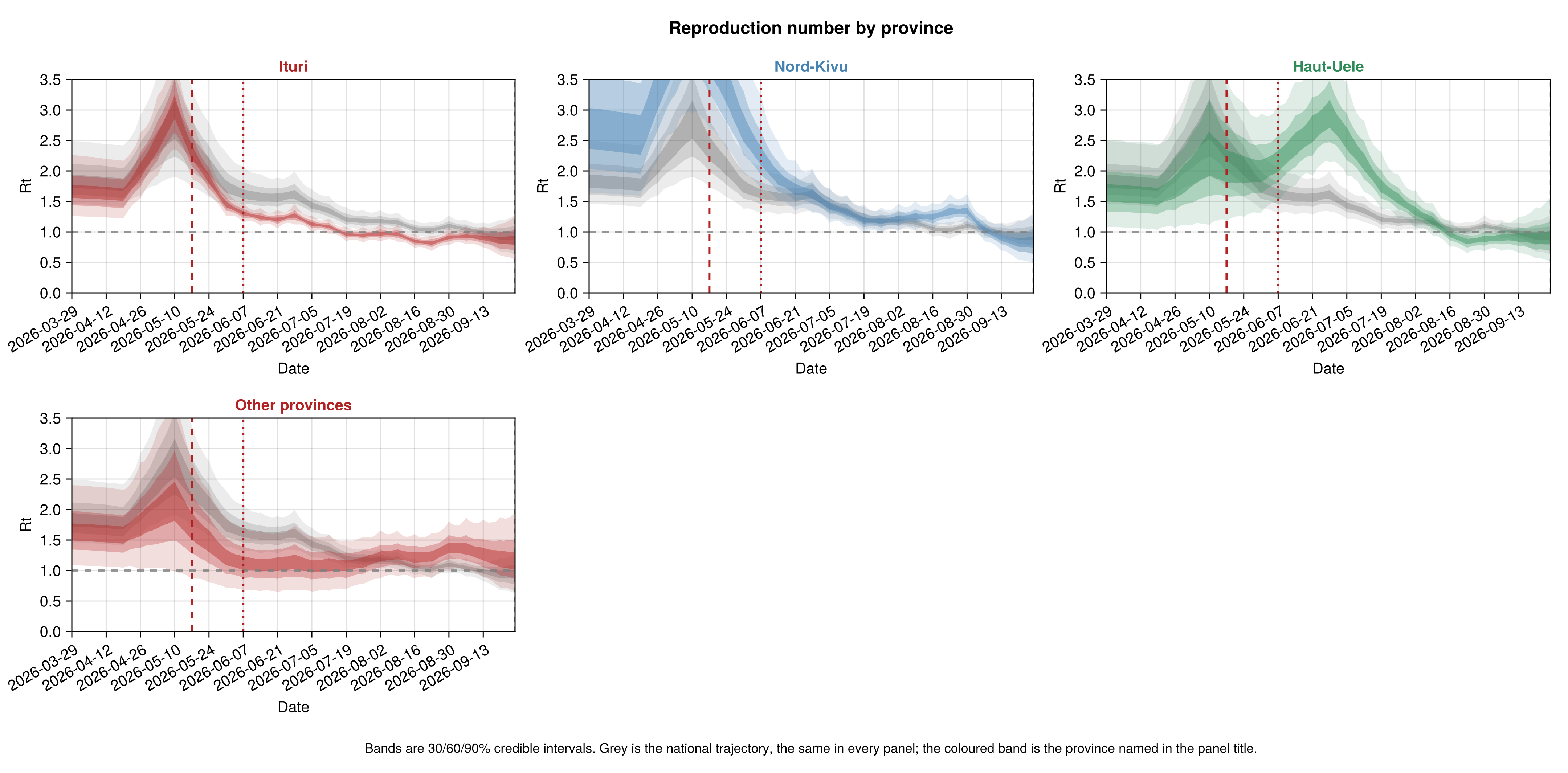
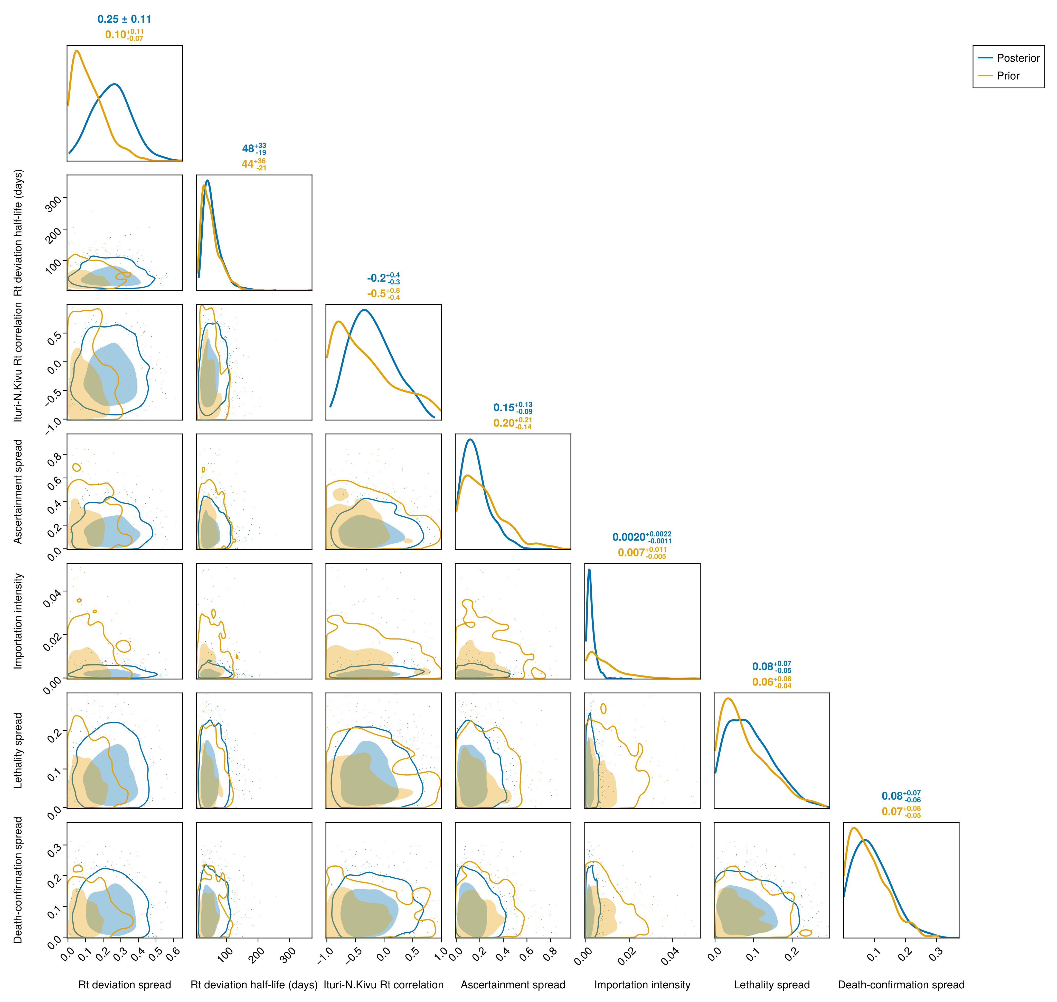
The spread of the provinces' log-Rt deviations is the spatial diagnostic. The prior admits real divergence, with a 26% prior probability that the Ituri to Nord-Kivu ratio moves by more than 25% over the window. With four patches and the pooled one carrying almost no signal the cross-province correlation is not identified, and it tracks its prior. It is the correlation of the provinces' deviation innovations, which sum to zero, so it leans negative. With equal spreads each province's correlations with the other three average −1/3.

Spatial hyperparameter summary table

# Labels for the spatial hyperparameters, shared by this table and the pair
# plot against their prior below.
spatial_labels = Dict(
    :region_sd => "Rt deviation spread",
    :region_halflife => "Rt deviation half-life (days)",
    :region_corr_primary_secondary => "Ituri-N.Kivu Rt correlation",
    :province_ascertainment_sd => "Ascertainment spread",
    :importation_epsilon => "Importation intensity",
    :province_cfr_sd => "Lethality spread",
    :province_death_ascertainment_sd => "Death-confirmation spread"
)
spatial_hyper_table = summary_table(
    chn_joint,
    [
        :region_sd, :region_halflife, :region_corr_primary_secondary,
        :province_ascertainment_sd,
    ];
    digits = 3, labels = spatial_labels
);

4×7 DataFrame

Row	Quantity	Lower 90%	Lower 60%	Lower 30%	Upper 30%	Upper 60%	Upper 90%
	String	Float64	Float64	Float64	Float64	Float64	Float64
1	Rt deviation spread	0.072	0.154	0.206	0.289	0.336	0.423
2	Rt deviation half-life (days)	23.563	32.159	40.187	58.053	74.852	110.368
3	Ituri-N.Kivu Rt correlation	-0.738	-0.536	-0.385	-0.087	0.129	0.489
4	Ascertainment spread	0.016	0.072	0.111	0.194	0.255	0.405

Case-fatality ratio by province

Whether the case-fatality ratio varies by province, set against the national ratios in the confirmed case-fatality ratio. Only the product of a province's lethality and death confirmation is identified, and the province compositions Methods section says how the priors split it.

Province case-fatality spread

province_cfr_spread = summary_table(
    chn_joint,
    [:province_cfr_sd, :province_death_ascertainment_sd];
    digits = 3, labels = spatial_labels
);

2×7 DataFrame

Row	Quantity	Lower 90%	Lower 60%	Lower 30%	Upper 30%	Upper 60%	Upper 90%
	String	Float64	Float64	Float64	Float64	Float64	Float64
1	Lethality spread	0.012	0.039	0.062	0.111	0.141	0.2
2	Death-confirmation spread	0.009	0.038	0.063	0.11	0.141	0.205

Province case-fatality table

confirmed_cfr = delay_corrected_confirmed_cfr(
    chn_joint;
    obs_confirmed = obs.confirmed_cases,
    obs_confirmed_deaths = obs.confirmed_deaths
);
province_cfr = province_cfr_table(
    chn_joint, confirmed_cfr;
    province_cases = vec(sum(province_cases.increments; dims = 2)),
    province_deaths = vec(sum(province_deaths.increments; dims = 2)),
    n_patches = N_PATCHES
);

4×4 DataFrame

Row	Province	Naive observed confirmed ratio	Delay-corrected confirmed CFR	Structural (infection-based) CFR
	String	String	String	String
1	Ituri	46.0%	41.7% (35.6–49.0%)	46.0% (34.4–59.9%)
2	Nord-Kivu	59.5%	59.1% (49.9–70.2%)	50.0% (37.5–67.2%)
3	Haut-Uele	42.1%	41.9% (34.7–50.7%)	45.4% (34.6–58.8%)
4	Other provinces	37.9%	47.0% (36.0–61.3%)	46.6% (34.4–59.8%)

Province parameters against their priors

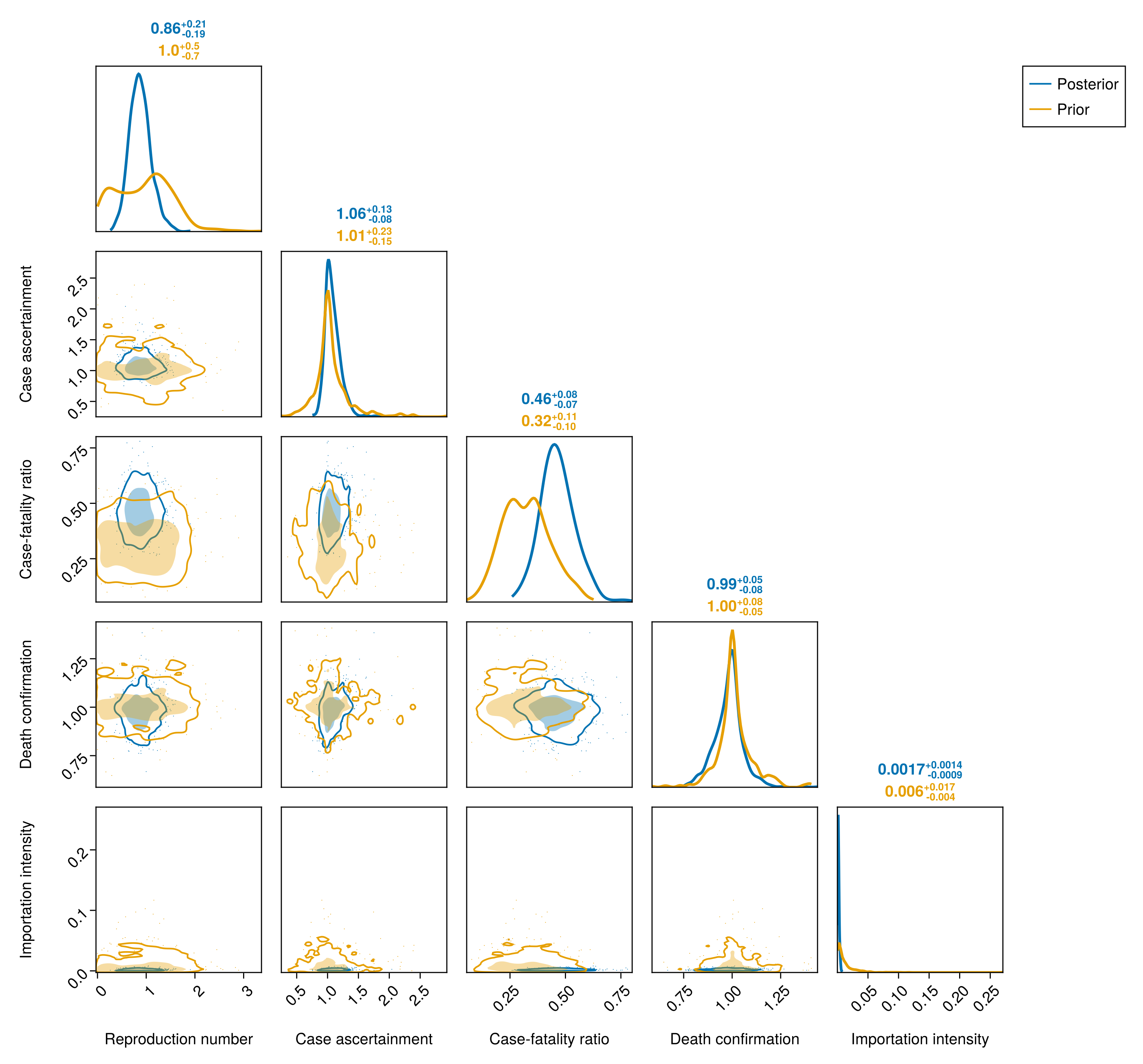
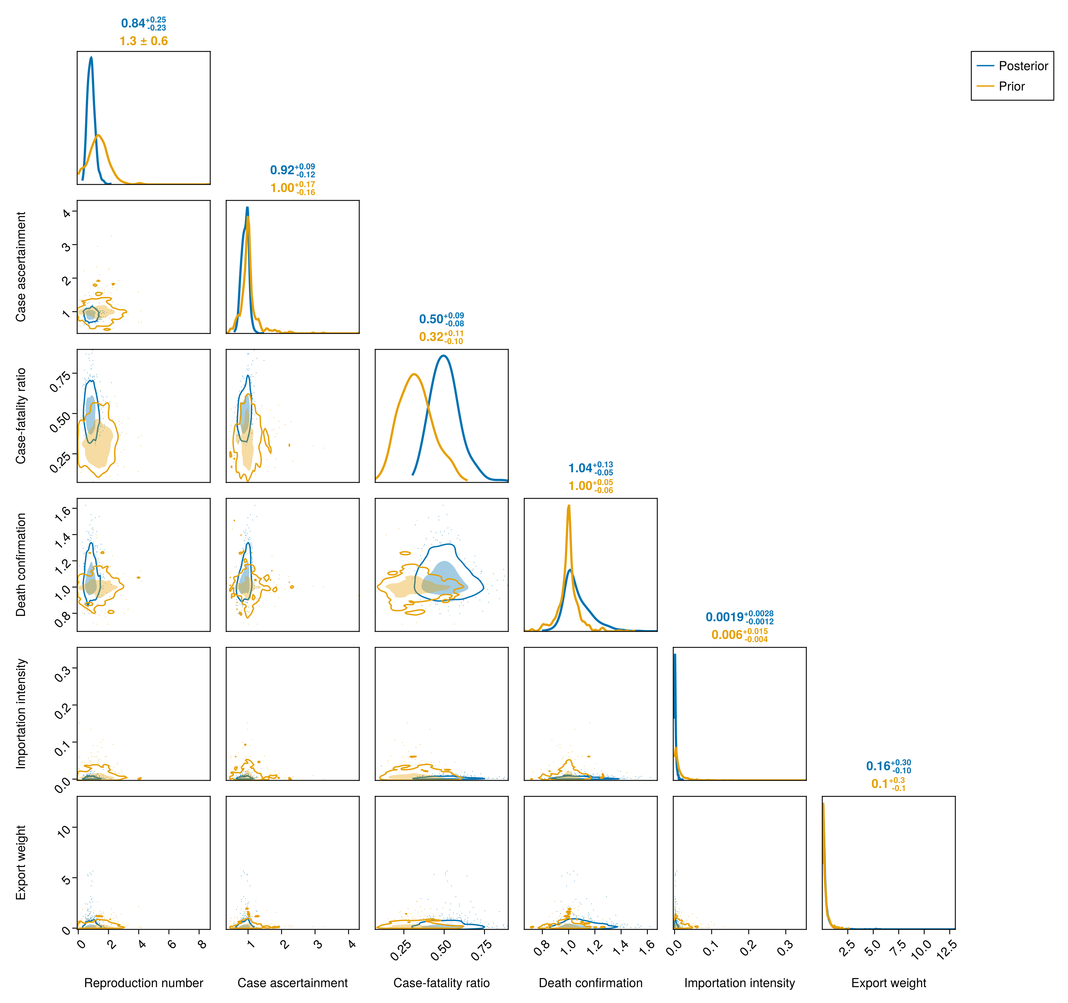
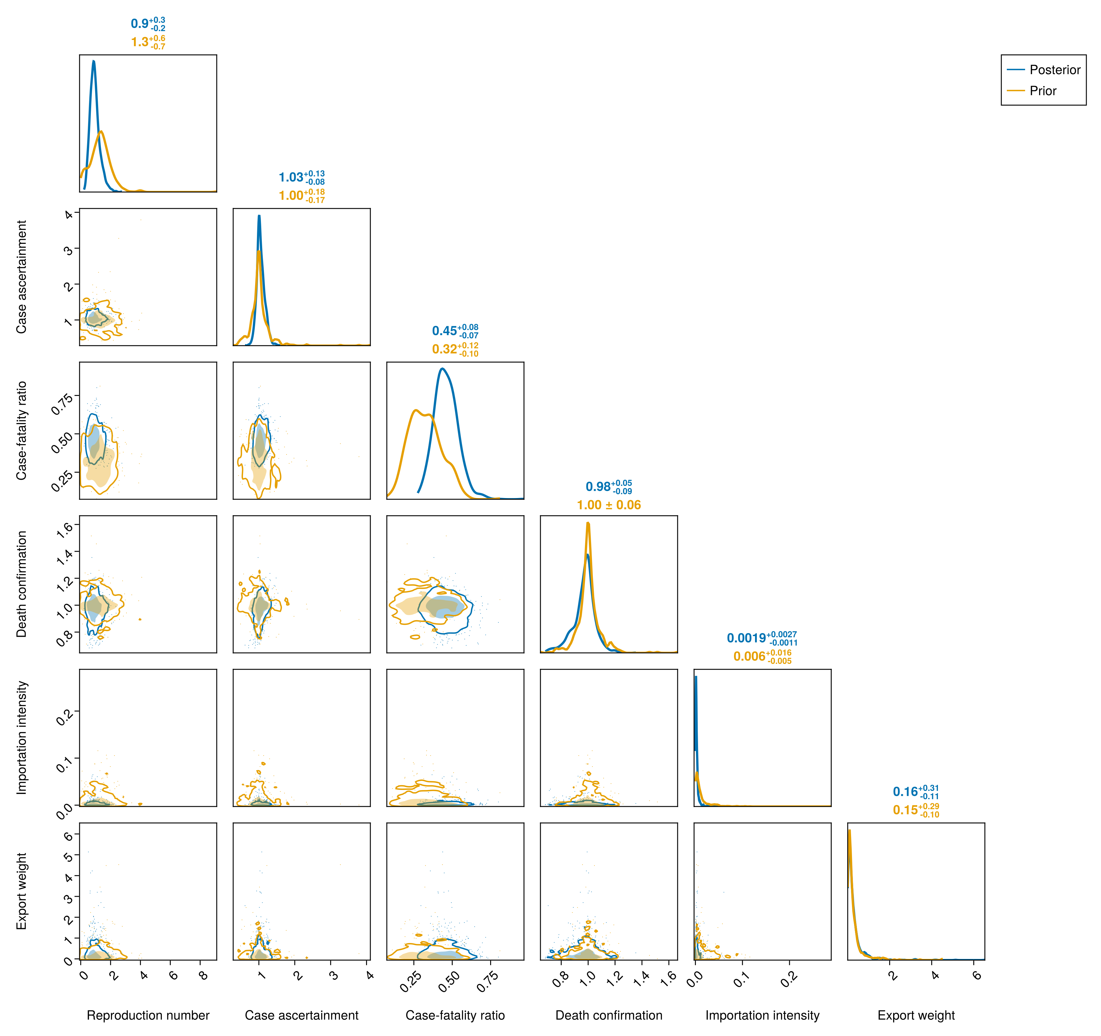
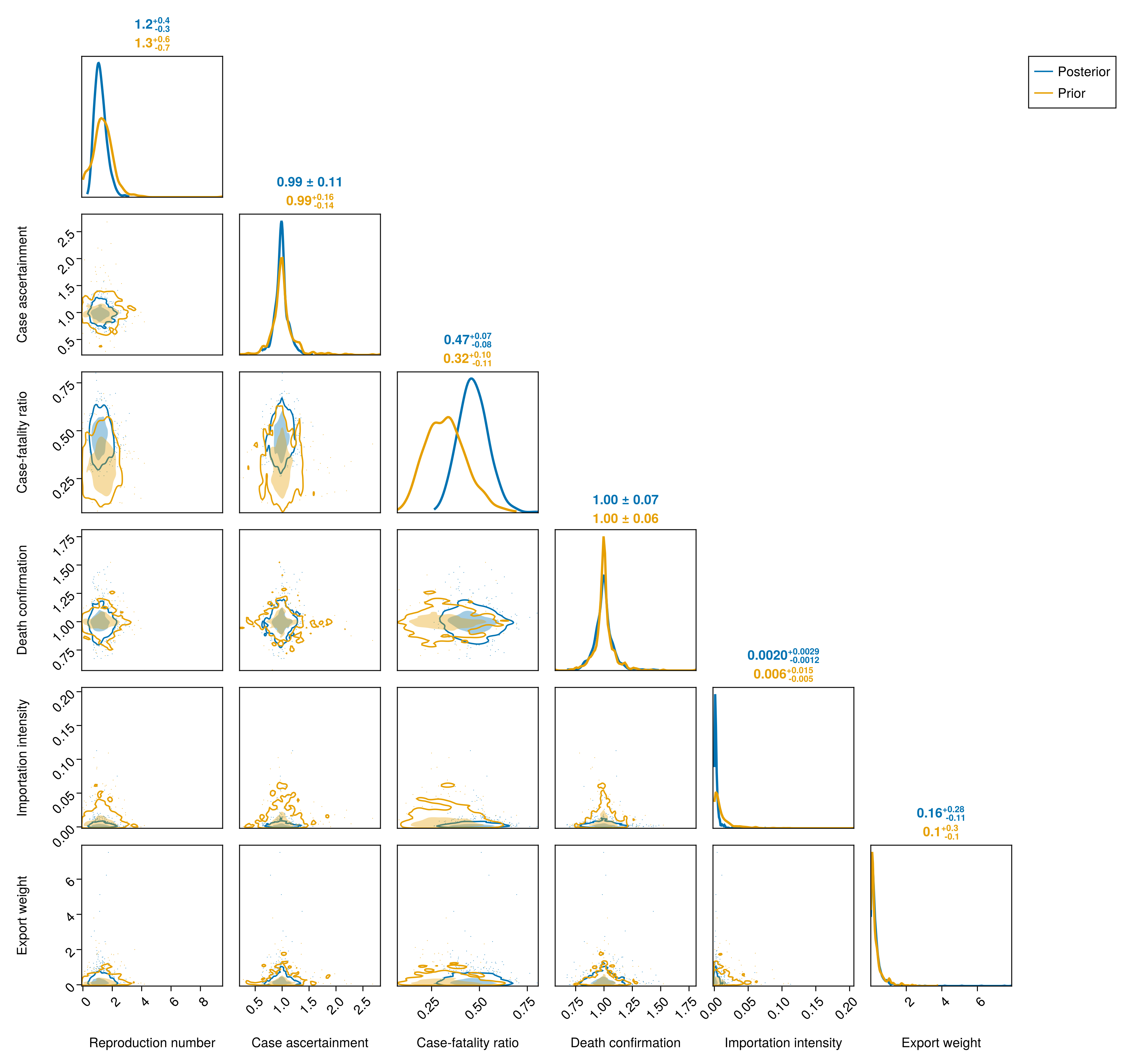
The pair plots below set the posterior of the province parameters against their prior. The prior is the four-patch model's, as the shared prior draws carry no province parameters.

Draw from the patch model's prior

prior_patch_chn = patch_prior_draws(obs);

The first pair plot covers the spatial hyperparameters: the spread, half-life and correlation of the Rt deviations, the spread of case ascertainment, the importation intensity, and the spreads of lethality and death confirmation.

Spatial hyperparameter pair plot (prior overlaid)

spatial_pair_fig = plot_pair(
    chn_joint,
    [
        :region_sd, :region_halflife, :region_corr_primary_secondary,
        :province_ascertainment_sd, :importation_epsilon, :province_cfr_sd,
        :province_death_ascertainment_sd,
    ];
    prior = prior_patch_chn, labels = spatial_labels
);

The pair plots below take one province at a time. Each sets the reproduction number at the cut-off against the relative case ascertainment, the case-fatality ratio against the relative death confirmation, and the province's importation intensity against its export weight relative to Ituri. Each pair is identified only as a product, so a ridge between the two is expected and its position along the ridge is set by the prior.

Compute the per-province pair plots

province_pair_labels = Dict(
    :R_T_patch => "Reproduction number",
    :province_ascertainment => "Case ascertainment",
    :CFR_patch => "Case-fatality ratio",
    :province_death_ascertainment => "Death confirmation",
    :importation_epsilon_patch => "Importation intensity",
    :export_weight => "Export weight"
)
# Ituri is the export reference, its weight fixed at one, so its pair plot
# leaves the weight out.
province_pair_figs = [
    plot_pair(
        chn_joint,
        [
            :R_T_patch, :province_ascertainment,
            :CFR_patch, :province_death_ascertainment,
            :importation_epsilon_patch,
            (p == 1 ? () : (:export_weight,))...,
        ];
        patch = p, prior = prior_patch_chn, labels = province_pair_labels
    )
        for p in 1:N_PATCHES
];

Ituri pair plot (prior overlaid)

Nord-Kivu pair plot (prior overlaid)

Haut-Uele pair plot (prior overlaid)

Other provinces pair plot (prior overlaid)

Composition checks

Whether the model reproduces each province's observed share of the national total is on the in-sample checks page.

Data currency

The province blocks are the situation reports' provincial tables: confirmed cases, confirmed deaths and the 24h laboratory volumes. Each is read here against the cut-off, so a block that stops updating shows as a date before it rather than as a flat series.

Province block currency

# Every province block whose last vintage falls before the cut-off, from
# the shared stream registry rather than a per-page list of dates. The
# grace the national table allows is not applied here: one vintage behind
# is already worth reading.
province_currency = let
    status = stream_report_status(obs; stratum = :province)
    behind = status[[ismissing(d) || d > 0 for d in status.days_since], :]
    isempty(behind) ?
        Markdown.parse(
            "Every province block reports to the cut-off, $(obs.cutoff)."
        ) :
        MarkdownTable(
            DataFrame(
                "Block" => behind.label,
                "Last reported" => [
                    ismissing(d) ? "never" : string(d)
                    for d in behind.last_date
                ],
                "Days before cut-off" => [
                    ismissing(d) ? "-" : string(d)
                    for d in behind.days_since
                ]
            )
        )
end;

Every province block reports to the cut-off, 2026-09-26.

Saving province assets

The summary dashboard shows the province comparison and the reproduction number by province, so they are written here rather than on the National page.

Write the province dashboard assets

dashboard_dir = joinpath(
    pkgdir(BVDOutbreakSize), "docs", "src", "summary_assets"
)
mkpath(dashboard_dir)
CairoMakie.save(joinpath(dashboard_dir, "rt_provinces.png"), province_rt_fig)
open(joinpath(dashboard_dir, "provinces.md"), "w") do io
    print(io, province_headline_md)
end

---

The full analysis code, data and model definitions are in the epiforecasts/BVDOutbreakSize repository.