Health-zone estimates
Each patch of the headline joint fit split across its health zones: the reproduction number, the share of the patch, the one-week forecast and the probability of at least a few cases, zone by zone. The health-zone model on the methods page gives the maths. This page carries its results, the checks of the fit and the interactive map. The change in each zone's estimate over the past week has its own section below. The one-week zone forecast is on the health-zone forecasts page and its scores in the health-zone forecast evaluation.
Load packages, data and fitted chains
# Shared setup: packages, observations and the fit registry. See
# `docs/pages/_setup.jl`.
using BVDOutbreakSize
include(joinpath(pkgdir(BVDOutbreakSize), "docs", "pages", "_setup.jl"))
validation_forecast_from (generic function with 1 method)# The fits this page reads, loaded from the cache here: the headline joint,
# the zone fit melded from it, and the frozen zone fit the week-on-week
# comparison reads.
chn_joint = load_fit("joint");
chn_local = load_fit("local");
frozen_local = load_fit("local_frozen_validation");
# The zone stage's fixed inputs with the joint's forecast, and the frozen
# fit's inputs for the comparison below, both from the shared setup, so the
# health-zone forecast page draws the same forecast from the same inputs.
zone_inputs = zone_stage_inputs(; forecast = true);
zone_patch = zone_inputs.patch_of_zone;
frozen_zone_inputs = frozen_zone_stage_inputs();Last updated: 30 September 2026.
Data as of: 26 September 2026.
Estimates by zone
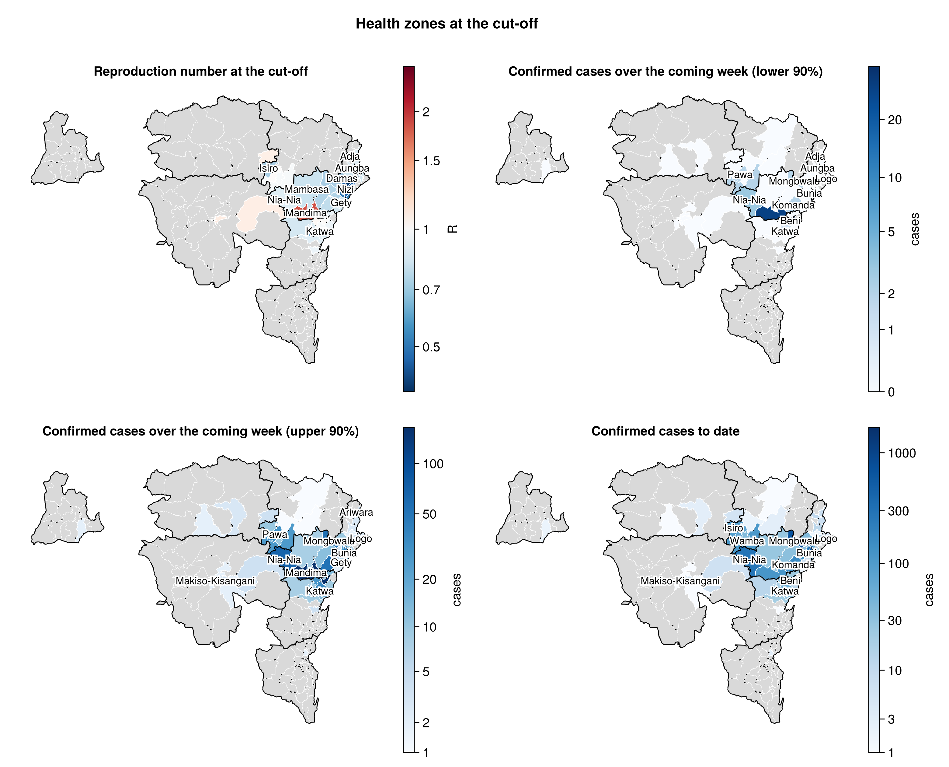
The maps below show, for the health-zone model, the reproduction number at the cut-off, the bounds of the 90% interval on the forecast confirmed cases over the coming week, and the confirmed cases to date, zone by zone. The forecast is mapped as its two bounds rather than a single number, so a zone's colour reads as a range. On the reproduction-number map a zone whose 90% interval straddles one is washed towards white. Zones with no confirmed case, or too few infections for a reproduction number, are grey. The four maps share the zone boundaries. A zone's forecast can be read against its reproduction number and its cases to date. The interactive map below adds the probability of at least
Health-zone post-processing
# The geojson keys a zone without the province prefix the manifest carries.
zone_map_keys = [
    String(last(split(k, "."; limit = 2)))
        for k in zone_inputs.zone_keys
];
# Daily zone reproduction numbers over the zone grid, each zone draw on
# its own draw of the patch trajectory so the patch uncertainty is
# carried, and the cut-off values the map and ranking read. A zone's
# reproduction number is reported from the day its cumulative infections
# reach the floor in the median draw.
zone_rt_traj = reconstruct_zone_rt(chn_local, zone_inputs);
zone_RT_finite = [filter(isfinite, m[:, obs.n]) for m in zone_rt_traj];
zone_RT_reported = findall(!isempty, zone_RT_finite);
zone_share_T = let vs = vec(collect(chn_local[:share_T_zone]))
    [Float64[v[z] for v in vs] for z in eachindex(zone_map_keys)]
end;
_zq(v, p) = quantile(v, p)
# The one-week zone forecast drawn from the zone model, and the
# probability of at least K cases per zone from the same draws.
zone_fc = zone_forecast(chn_local, zone_inputs);
zone_fc_draws = zone_forecast_draws(zone_fc, zone_inputs);
ZONE_THRESHOLDS = (1, 5, 10, 20)
zone_fc_probs = zone_forecast_probabilities(
    zone_fc, zone_inputs; thresholds = ZONE_THRESHOLDS, draws = zone_fc_draws
);
zone_overview = zone_overview_table(chn_local, zone_inputs);
# Cases allocated to each zone over the past one, two and four weeks,
# and the last vintage on which each zone's count rose.
zone_recent = Dict(
    w => zone_recent_cases(zone_inputs; window = w) for w in (7, 14, 28)
);
zone_last_case = zone_last_case_dates(zone_inputs);

zone_map_fig = plot_zone_map_panels(
    [
        (;
            values = [median(zone_RT_finite[z]) for z in zone_RT_reported],
            zones = zone_map_keys[zone_RT_reported],
            lower = [_zq(zone_RT_finite[z], 0.05) for z in zone_RT_reported],
            upper = [_zq(zone_RT_finite[z], 0.95) for z in zone_RT_reported],
            diverging_at = 1.0, scale = log10,
            title = "Reproduction number at the cut-off",
            colorbar_label = "R",
        ),
        (;
            values = [_zq(v, 0.05) for v in zone_fc_draws.zones],
            zones = zone_map_keys, scale = CairoMakie.Makie.pseudolog10,
            title = "Confirmed cases over the coming week (lower 90%)",
            colorbar_label = "cases",
        ),
        (;
            values = [_zq(v, 0.95) for v in zone_fc_draws.zones],
            zones = zone_map_keys, scale = CairoMakie.Makie.pseudolog10,
            title = "Confirmed cases over the coming week (upper 90%)",
            colorbar_label = "cases",
        ),
        (;
            values = Float64.(zone_inputs.cumulative), zones = zone_map_keys,
            scale = CairoMakie.Makie.pseudolog10,
            title = "Confirmed cases to date", colorbar_label = "cases",
        ),
    ];
    ncols = 2, title = "Health zones at the cut-off"
);
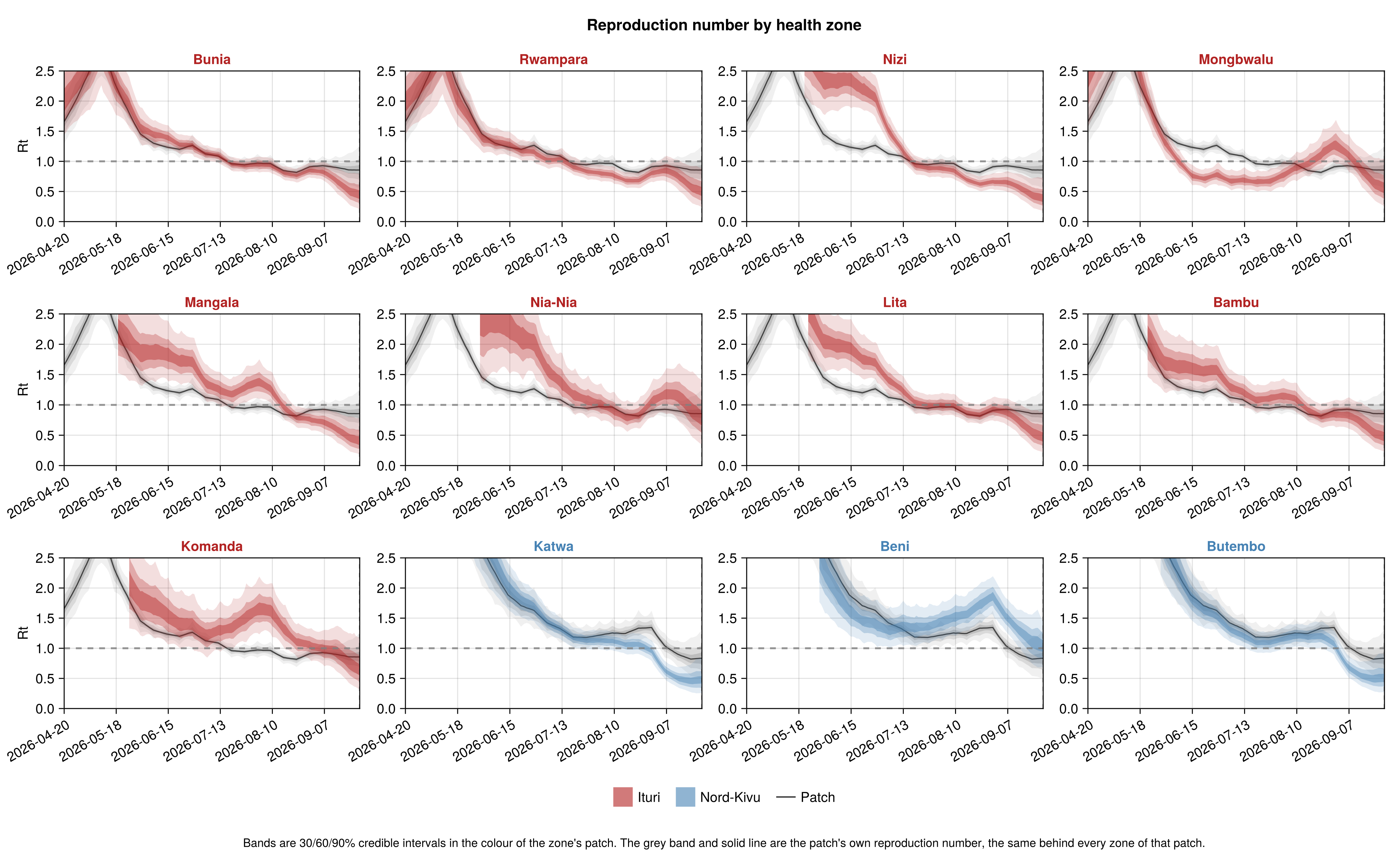
The panels below trace the reproduction number of the twelve zones with most confirmed cases, each against its patch's own implied reproduction number in grey. Where a zone's line departs from the grey patch line, the gap is the zone's fitted deviation from its patch.
Zone reproduction-number trajectories
# Each patch's implied reproduction number from the joint draws with the
# same generation interval the zone stage fixes, so the grey reference is
# the quantity the zone values average to.
zone_grid = zone_inputs.t0:obs.n
_patch_infection_draws = vec(collect(chn_joint[:infections_patch]));
patch_implied_rt = [
    let m = Matrix{Float64}(
            undef,
            length(_patch_infection_draws), obs.n
        )
        for (i, v) in enumerate(_patch_infection_draws)
            I = reshape(Float64.(v), N_PATCHES, obs.n)
            m[i, :] .= implied_national_Rt(I[p, :], zone_inputs.g)
        end
        m
    end
        for p in 1:N_PATCHES
];
zone_rt_fig = plot_rt_zones(
    [replace(m[:, zone_grid], NaN => missing) for m in zone_rt_traj],
    zone_inputs.zone_labels, zone_patch;
    patch_labels = zone_inputs.patch_labels,
    dates = grid_date.(zone_grid), as_of_date = obs.cutoff,
    cumulative = zone_inputs.cumulative, top = 12,
    patch_rt = [m[:, zone_grid] for m in patch_implied_rt]
);
The ranking below orders the zones by the posterior probability that their reproduction number exceeds one. A zone whose reproduction number is from its province, not modelled separately, is drawn hollow in grey.
Zone ranking
zone_ranking_fig = plot_zone_ranking(
    zone_overview;
    patch_labels = zone_inputs.patch_labels
);
# The overview as displayed: the interval strings, without the numeric
# columns the figure reads.
zone_overview_display = let d = zone_overview[
        :,
        [:zone, :patch, :cases, :share, :R_T, :p_R_above_1, :delta_T],
    ]
    d[!, "R modelled separately"] = [
        w ? "yes" : "no" for w in zone_overview.walking
    ]
    d
end;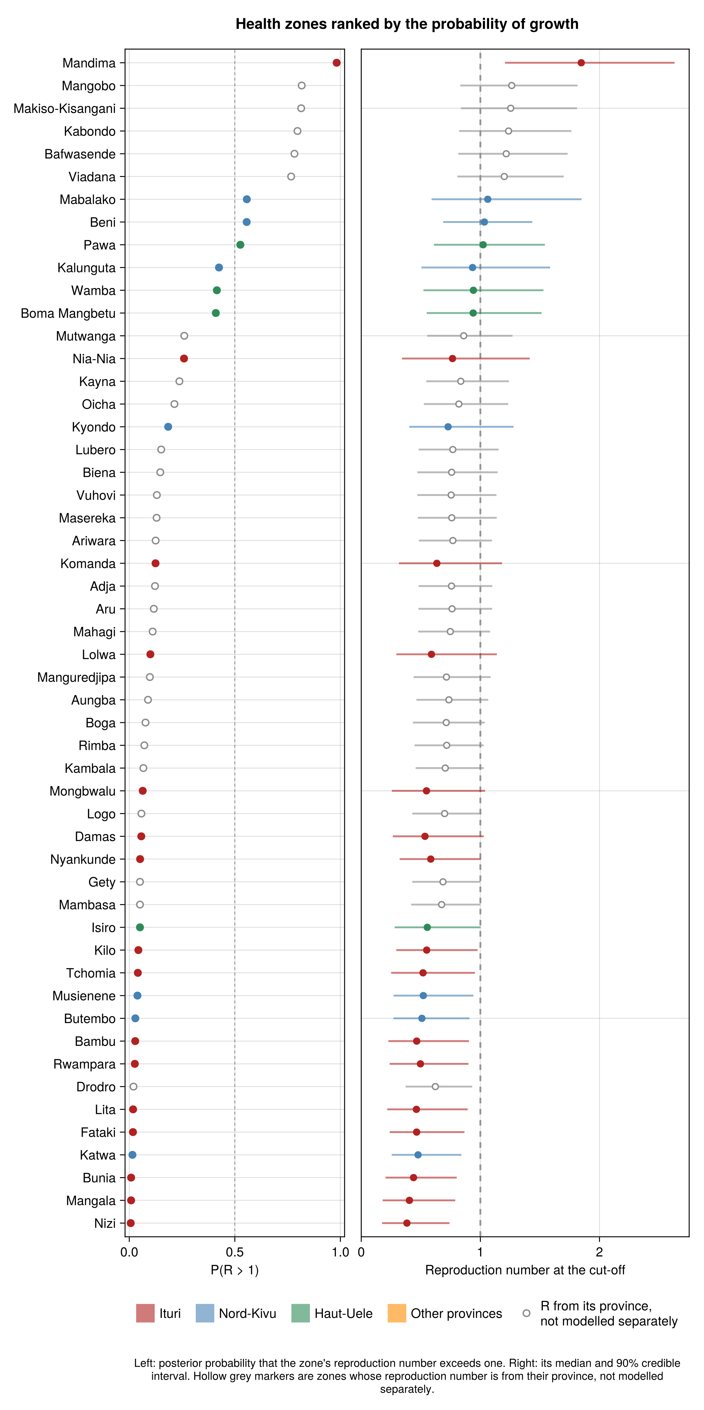
The table gives the twenty highest-ranked zones: the confirmed cases to date, the zone's share of its patch's infections at the cut-off in percent, its reproduction number, the probability that it exceeds one, its log-transmission deviation at the cut-off and whether its reproduction number is modelled separately. A zone whose reproduction number is not modelled separately takes it from its province. The share, the reproduction number and the deviation are each a median with a 90% interval. Every zone is listed in the fold below it.
| zone | patch | cases | share | R_T | p_R_above_1 | delta_T | R modelled separately |
|---|---|---|---|---|---|---|---|
| Mandima | Ituri | 118 | 50.7 (25.2–73.9) | 1.85 (1.21–2.63) | 0.98 | 1.38 (0.72–2.09) | yes |
| Beni | Nord-Kivu | 329 | 61.6 (43.6–76.2) | 1.03 (0.69–1.44) | 0.56 | 0.5 (0.08–0.97) | yes |
| Mabalako | Nord-Kivu | 31 | 6.0 (2.4–14.5) | 1.06 (0.59–1.85) | 0.56 | 0.49 (0.05–1.03) | yes |
| Pawa | Haut-Uele | 77 | 48.6 (27.9–69.3) | 1.02 (0.61–1.54) | 0.53 | 0.3 (-0.02–0.66) | yes |
| Kalunguta | Nord-Kivu | 51 | 6.0 (2.8–13.6) | 0.93 (0.5–1.59) | 0.42 | 0.34 (-0.03–0.74) | yes |
| Wamba | Haut-Uele | 109 | 29.1 (13.9–51.6) | 0.94 (0.52–1.53) | 0.42 | 0.21 (-0.13–0.65) | yes |
| Boma Mangbetu | Haut-Uele | 39 | 10.0 (4.6–21.5) | 0.94 (0.55–1.51) | 0.41 | 0.15 (-0.16–0.5) | yes |
| Nia-Nia | Ituri | 284 | 8.7 (3.2–21.5) | 0.77 (0.34–1.41) | 0.26 | 0.47 (-0.14–1.15) | yes |
| Kyondo | Nord-Kivu | 33 | 1.6 (0.7–3.8) | 0.73 (0.4–1.28) | 0.18 | -0.02 (-0.5–0.43) | yes |
| Komanda | Ituri | 166 | 6.3 (2.5–15.0) | 0.63 (0.32–1.18) | 0.12 | 0.28 (-0.28–0.85) | yes |
| Lolwa | Ituri | 33 | 0.4 (0.1–1.5) | 0.59 (0.3–1.14) | 0.1 | 0.14 (-0.42–0.77) | yes |
| Damas | Ituri | 40 | 0.2 (0.1–0.8) | 0.53 (0.26–1.03) | 0.06 | -0.11 (-0.71–0.49) | yes |
| Mongbwalu | Ituri | 697 | 5.0 (2.0–12.1) | 0.55 (0.26–1.04) | 0.06 | 0.14 (-0.39–0.68) | yes |
| Nyankunde | Ituri | 127 | 0.2 (0.1–0.6) | 0.58 (0.32–1.0) | 0.05 | -0.14 (-0.72–0.41) | yes |
| Isiro | Haut-Uele | 100 | 7.2 (2.8–16.4) | 0.55 (0.28–1.0) | 0.05 | -0.39 (-0.95–0.03) | yes |
| Kilo | Ituri | 35 | 0.1 (0.0–0.4) | 0.55 (0.29–0.98) | 0.04 | -0.13 (-0.61–0.37) | yes |
| Tchomia | Ituri | 76 | 0.4 (0.1–1.3) | 0.52 (0.25–0.95) | 0.04 | -0.04 (-0.54–0.43) | yes |
| Musienene | Nord-Kivu | 121 | 2.0 (0.9–4.5) | 0.52 (0.27–0.94) | 0.04 | -0.33 (-0.81–0.1) | yes |
| Bambu | Ituri | 201 | 1.3 (0.5–3.4) | 0.47 (0.23–0.9) | 0.03 | -0.05 (-0.46–0.37) | yes |
| Rwampara | Ituri | 1078 | 3.4 (1.4–8.4) | 0.5 (0.24–0.9) | 0.03 | 0.0 (-0.4–0.41) | yes |
All health zones
| zone | patch | cases | share | R_T | p_R_above_1 | delta_T | R modelled separately |
|---|---|---|---|---|---|---|---|
| Mandima | Ituri | 118 | 50.7 (25.2–73.9) | 1.85 (1.21–2.63) | 0.98 | 1.38 (0.72–2.09) | yes |
| Beni | Nord-Kivu | 329 | 61.6 (43.6–76.2) | 1.03 (0.69–1.44) | 0.56 | 0.5 (0.08–0.97) | yes |
| Mabalako | Nord-Kivu | 31 | 6.0 (2.4–14.5) | 1.06 (0.59–1.85) | 0.56 | 0.49 (0.05–1.03) | yes |
| Pawa | Haut-Uele | 77 | 48.6 (27.9–69.3) | 1.02 (0.61–1.54) | 0.53 | 0.3 (-0.02–0.66) | yes |
| Kalunguta | Nord-Kivu | 51 | 6.0 (2.8–13.6) | 0.93 (0.5–1.59) | 0.42 | 0.34 (-0.03–0.74) | yes |
| Wamba | Haut-Uele | 109 | 29.1 (13.9–51.6) | 0.94 (0.52–1.53) | 0.42 | 0.21 (-0.13–0.65) | yes |
| Boma Mangbetu | Haut-Uele | 39 | 10.0 (4.6–21.5) | 0.94 (0.55–1.51) | 0.41 | 0.15 (-0.16–0.5) | yes |
| Nia-Nia | Ituri | 284 | 8.7 (3.2–21.5) | 0.77 (0.34–1.41) | 0.26 | 0.47 (-0.14–1.15) | yes |
| Kyondo | Nord-Kivu | 33 | 1.6 (0.7–3.8) | 0.73 (0.4–1.28) | 0.18 | -0.02 (-0.5–0.43) | yes |
| Komanda | Ituri | 166 | 6.3 (2.5–15.0) | 0.63 (0.32–1.18) | 0.12 | 0.28 (-0.28–0.85) | yes |
| Lolwa | Ituri | 33 | 0.4 (0.1–1.5) | 0.59 (0.3–1.14) | 0.1 | 0.14 (-0.42–0.77) | yes |
| Damas | Ituri | 40 | 0.2 (0.1–0.8) | 0.53 (0.26–1.03) | 0.06 | -0.11 (-0.71–0.49) | yes |
| Mongbwalu | Ituri | 697 | 5.0 (2.0–12.1) | 0.55 (0.26–1.04) | 0.06 | 0.14 (-0.39–0.68) | yes |
| Nyankunde | Ituri | 127 | 0.2 (0.1–0.6) | 0.58 (0.32–1.0) | 0.05 | -0.14 (-0.72–0.41) | yes |
| Isiro | Haut-Uele | 100 | 7.2 (2.8–16.4) | 0.55 (0.28–1.0) | 0.05 | -0.39 (-0.95–0.03) | yes |
| Kilo | Ituri | 35 | 0.1 (0.0–0.4) | 0.55 (0.29–0.98) | 0.04 | -0.13 (-0.61–0.37) | yes |
| Tchomia | Ituri | 76 | 0.4 (0.1–1.3) | 0.52 (0.25–0.95) | 0.04 | -0.04 (-0.54–0.43) | yes |
| Musienene | Nord-Kivu | 121 | 2.0 (0.9–4.5) | 0.52 (0.27–0.94) | 0.04 | -0.33 (-0.81–0.1) | yes |
| Bambu | Ituri | 201 | 1.3 (0.5–3.4) | 0.47 (0.23–0.9) | 0.03 | -0.05 (-0.46–0.37) | yes |
| Rwampara | Ituri | 1078 | 3.4 (1.4–8.4) | 0.5 (0.24–0.9) | 0.03 | 0.0 (-0.4–0.41) | yes |
| Butembo | Nord-Kivu | 256 | 4.4 (2.1–8.5) | 0.51 (0.27–0.91) | 0.03 | -0.31 (-0.64–0.01) | yes |
| Fataki | Ituri | 82 | 0.3 (0.1–0.8) | 0.46 (0.24–0.87) | 0.02 | -0.31 (-0.9–0.24) | yes |
| Lita | Ituri | 283 | 2.3 (0.9–5.7) | 0.46 (0.22–0.89) | 0.02 | -0.05 (-0.46–0.39) | yes |
| Katwa | Nord-Kivu | 555 | 7.1 (3.6–13.2) | 0.48 (0.26–0.84) | 0.02 | -0.39 (-0.72–-0.09) | yes |
| Bunia | Ituri | 1697 | 8.6 (3.4–17.4) | 0.44 (0.2–0.8) | 0.01 | -0.1 (-0.48–0.27) | yes |
| Mangala | Ituri | 346 | 2.3 (0.9–5.4) | 0.4 (0.18–0.79) | 0.01 | -0.17 (-0.61–0.22) | yes |
| Nizi | Ituri | 771 | 1.9 (0.8–4.6) | 0.38 (0.17–0.74) | 0.01 | -0.25 (-0.63–0.16) | yes |
| Mangobo | Other provinces | 5 | 9.6 (5.6–17.1) | 1.26 (0.83–1.82) | 0.82 | 0.04 (0.0–0.12) | no |
| Makiso-Kisangani | Other provinces | 23 | 43.4 (30.8–57.4) | 1.25 (0.84–1.81) | 0.81 | 0.08 (0.03–0.19) | no |
| Kabondo | Other provinces | 5 | 7.2 (3.5–13.7) | 1.24 (0.82–1.76) | 0.8 | 0.03 (-0.02–0.1) | no |
| Bafwasende | Other provinces | 7 | 6.9 (2.9–15.1) | 1.22 (0.81–1.73) | 0.78 | 0.04 (-0.02–0.14) | no |
| Viadana | Other provinces | 6 | 6.6 (2.8–14.7) | 1.2 (0.81–1.7) | 0.77 | 0.02 (-0.05–0.1) | no |
| Mutwanga | Nord-Kivu | 12 | 0.9 (0.5–1.6) | 0.86 (0.55–1.27) | 0.26 | -0.05 (-0.18–-0.0) | no |
| Kayna | Nord-Kivu | 1 | 0.3 (0.2–0.6) | 0.84 (0.55–1.24) | 0.24 | -0.13 (-0.37–-0.03) | no |
| Oicha | Nord-Kivu | 24 | 1.6 (1.0–2.6) | 0.82 (0.53–1.23) | 0.21 | 0.0 (-0.06–0.05) | no |
| Biena | Nord-Kivu | 18 | 0.8 (0.4–1.4) | 0.76 (0.47–1.15) | 0.15 | 0.02 (-0.03–0.07) | no |
| Lubero | Nord-Kivu | 21 | 1.1 (0.6–1.8) | 0.77 (0.48–1.15) | 0.15 | -0.01 (-0.1–0.03) | no |
| Masereka | Nord-Kivu | 28 | 1.3 (0.7–2.2) | 0.76 (0.47–1.14) | 0.13 | -0.0 (-0.06–0.04) | no |
| Vuhovi | Nord-Kivu | 29 | 1.5 (0.8–2.5) | 0.75 (0.47–1.13) | 0.13 | 0.02 (-0.01–0.08) | no |
| Adja | Ituri | 11 | 0.1 (0.0–0.1) | 0.76 (0.48–1.1) | 0.12 | -0.1 (-0.33–-0.02) | no |
| Ariwara | Ituri | 8 | 0.2 (0.1–0.3) | 0.77 (0.48–1.1) | 0.12 | -0.09 (-0.31–-0.01) | no |
| Aru | Ituri | 8 | 0.2 (0.1–0.3) | 0.76 (0.48–1.1) | 0.12 | -0.12 (-0.35–-0.03) | no |
| Mahagi | Ituri | 4 | 0.2 (0.1–0.2) | 0.75 (0.48–1.08) | 0.11 | -0.12 (-0.37–-0.03) | no |
| Manguredjipa | Nord-Kivu | 13 | 0.7 (0.3–1.4) | 0.72 (0.44–1.09) | 0.1 | 0.06 (0.01–0.16) | no |
| Aungba | Ituri | 12 | 0.1 (0.1–0.2) | 0.74 (0.46–1.07) | 0.09 | -0.11 (-0.31–-0.03) | no |
| Boga | Ituri | 2 | 0.1 (0.1–0.2) | 0.71 (0.43–1.04) | 0.08 | -0.02 (-0.12–0.04) | no |
| Kambala | Ituri | 2 | 0.1 (0.1–0.2) | 0.71 (0.46–1.03) | 0.07 | -0.1 (-0.27–-0.02) | no |
| Rimba | Ituri | 12 | 0.2 (0.1–0.3) | 0.72 (0.45–1.03) | 0.07 | -0.1 (-0.32–-0.02) | no |
| Logo | Ituri | 13 | 0.2 (0.1–0.3) | 0.7 (0.43–1.01) | 0.06 | -0.08 (-0.26–-0.02) | no |
| Gety | Ituri | 7 | 0.2 (0.1–0.4) | 0.69 (0.43–1.0) | 0.05 | -0.04 (-0.16–0.01) | no |
| Mambasa | Ituri | 27 | 0.3 (0.2–0.6) | 0.67 (0.42–1.0) | 0.05 | 0.02 (-0.02–0.1) | no |
| Drodro | Ituri | 15 | 0.3 (0.2–0.6) | 0.62 (0.37–0.93) | 0.02 | -0.02 (-0.12–0.02) | no |
| Goma | Nord-Kivu | 1 | 0.2 (0.1–0.3) | NaN | -0.11 (-0.34–-0.02) | no | |
| Dungu | Haut-Uele | 1 | 0.5 (0.3–0.9) | NaN | -0.12 (-0.31–-0.04) | no | |
| Gombari | Haut-Uele | 3 | 0.5 (0.2–1.1) | NaN | -0.05 (-0.17–-0.0) | no | |
| Rungu | Haut-Uele | 2 | 0.9 (0.5–1.5) | NaN | -0.07 (-0.23–-0.01) | no | |
| Miti-Murhesa | Other provinces | 3 | 2.8 (1.0–6.3) | NaN | -0.08 (-0.25–-0.01) | no | |
| Lubunga | Other provinces | 1 | 3.9 (1.8–7.7) | NaN | 0.01 (-0.08–0.07) | no | |
| Tshopo | Other provinces | 1 | 2.5 (1.1–5.5) | NaN | -0.03 (-0.17–0.03) | no | |
| Wanie-Rukula | Other provinces | 1 | 2.4 (1.0–5.6) | NaN | -0.03 (-0.16–0.04) | no | |
| Buta | Other provinces | 1 | 2.6 (1.0–5.4) | NaN | -0.05 (-0.24–0.02) | no | |
| Ganga | Other provinces | 3 | 4.3 (1.7–9.6) | NaN | -0.0 (-0.11–0.07) | no | |
| Bulu | Other provinces | 2 | 2.2 (0.6–7.2) | NaN | 0.03 (-0.08–0.12) | no |
Composition checks
Whether the model reproduces each zone's observed share of its patch's confirmed cases and deaths is on the in-sample checks page.
Data currency
The zone blocks are the per-zone confirmed-case and confirmed-death tables of the situation reports. Each is read here against the cut-off, so a block that stops being picked up shows as a date before it rather than as a flat series.
Zone block currency
# Every zone block whose last vintage falls before the cut-off. The grace
# the national table allows is not applied here: one vintage behind is
# already worth reading.
zone_currency = let
    status = stream_report_status(obs; stratum = :zone)
    behind = status[[ismissing(d) || d > 0 for d in status.days_since], :]
    isempty(behind) ?
        Markdown.parse(
            "Every zone block reports to the cut-off, $(obs.cutoff)."
        ) :
        MarkdownTable(
            DataFrame(
                "Block" => behind.label,
                "Last reported" => [
                    ismissing(d) ? "never" : string(d)
                    for d in behind.last_date
                ],
                "Days before cut-off" => [
                    ismissing(d) ? "-" : string(d)
                    for d in behind.days_since
                ]
            )
        )
end;
Every zone block reports to the cut-off, 2026-09-26.
Health-zone fit diagnostics
The table gives the sampler diagnostics of the two zone fits: the worst R-hat and smallest effective sample sizes over every stored quantity but the zone reproduction number, and the divergences. Per chain it gives the fraction of iterations at the tree-depth cap, the energy fraction of missing information and the adapted step size. The per-zone R-hat and effective sample sizes of the cut-off reproduction number, share and deviation are in the fold. The rows whose reproduction number is modelled separately are the ones to read.
Zone fit diagnostics
_zone_per_chain(v) = join(string.(round.(v; sigdigits = 3)), " / ")
function _zone_sampler_row(label, chn)
    d = zone_sampler_diagnostics(chn)
    return (
        fit = label, max_rhat = round(d.max_rhat; digits = 3),
        min_ess_bulk = round(d.min_ess_bulk; digits = 0),
        min_ess_tail = round(d.min_ess_tail; digits = 0),
        divergences = d.n_divergent,
        depth_cap = _zone_per_chain(d.depth_cap_fraction),
        ebfmi = _zone_per_chain(d.ebfmi),
        step_size = _zone_per_chain(d.step_size),
    )
end
zone_sampler_table = DataFrame(
    [
        _zone_sampler_row("health zones", chn_local),
        _zone_sampler_row("health zones (frozen)", frozen_local.chn),
    ]
);
zone_diagnostics = let d = zone_diagnostics_table(chn_local, zone_inputs)
    for c in names(d)[3:end]
        d[!, c] = round.(d[!, c]; digits = startswith(c, "rhat") ? 3 : 0)
    end
    DataFrame(
        [
            n == "walking" ?
                "R modelled separately" => [w ? "yes" : "no" for w in d[!, n]] :
                n => d[!, n]
                for n in names(d)
        ]
    )
end;| fit | max_rhat | min_ess_bulk | min_ess_tail | divergences | depth_cap | ebfmi | step_size |
|---|---|---|---|---|---|---|---|
| health zones | 1.027 | 146 | 109 | 0 | 0.0 / 0.0 | 0.857 / 0.902 | 0.0099 / 0.0104 |
| health zones (frozen) | 1.019 | 214 | 251 | 0 | 0.0 / 0.0 | 0.966 / 0.917 | 0.00963 / 0.0113 |
Per-zone R-hat and effective sample sizes
| zone | R modelled separately | rhat_R_T | ess_bulk_R_T | ess_tail_R_T | rhat_share_T | ess_bulk_share_T | ess_tail_share_T | rhat_delta_T | ess_bulk_delta_T | ess_tail_delta_T |
|---|---|---|---|---|---|---|---|---|---|---|
| Adja | no | NaN | NaN | NaN | 1 | 1252 | 1268 | 1.003 | 1364 | 1121 |
| Ariwara | no | NaN | NaN | NaN | 1.001 | 1226 | 1095 | 1.001 | 1389 | 1434 |
| Aru | no | NaN | NaN | NaN | 1 | 1128 | 1207 | 0.999 | 1098 | 1275 |
| Aungba | no | NaN | NaN | NaN | 1.001 | 1208 | 1179 | 1.001 | 1063 | 996 |
| Bambu | yes | 1 | 2304 | 1227 | 1 | 2140 | 1430 | 1.001 | 2940 | 1341 |
| Boga | no | NaN | NaN | NaN | 1.001 | 1439 | 1345 | 1.001 | 1876 | 1013 |
| Bunia | yes | 1 | 1961 | 1005 | 1.001 | 1444 | 938 | 1 | 2698 | 1030 |
| Damas | yes | 1.001 | 2702 | 1208 | 1.001 | 1794 | 1508 | 1 | 3270 | 1176 |
| Drodro | no | 1.008 | 1952 | 1289 | 1.001 | 1440 | 1379 | 1 | 1176 | 1160 |
| Fataki | yes | 1.002 | 2003 | 1386 | 1.001 | 1759 | 1497 | 1.002 | 2635 | 1337 |
| Gety | no | NaN | NaN | NaN | 1.001 | 1228 | 1194 | 1 | 1486 | 1166 |
| Kambala | no | NaN | NaN | NaN | 1.001 | 1286 | 1203 | 1 | 939 | 1111 |
| Kilo | yes | 1.003 | 1864 | 1214 | 1.001 | 1816 | 1198 | 1.002 | 3405 | 1293 |
| Komanda | yes | 1 | 2458 | 1021 | 1 | 2030 | 1407 | 1.001 | 2951 | 1449 |
| Lita | yes | 1 | 2140 | 1097 | 1.001 | 2104 | 1247 | 1.005 | 2713 | 1224 |
| Logo | no | 1.008 | 1821 | 1328 | 1.003 | 1237 | 1393 | 1.001 | 857 | 1041 |
| Lolwa | yes | 1 | 2749 | 1190 | 1.01 | 1958 | 1491 | 1.001 | 3510 | 1372 |
| Mahagi | no | NaN | NaN | NaN | 1.001 | 1147 | 1242 | 1.001 | 966 | 1184 |
| Mambasa | no | 1.003 | 1750 | 1321 | 1.003 | 1373 | 874 | 1.001 | 1438 | 1073 |
| Mandima | yes | 1 | 1989 | 1195 | 1.001 | 1915 | 1367 | 1 | 2172 | 1216 |
| Mangala | yes | 1 | 2151 | 1440 | 1.001 | 1800 | 1341 | 1.003 | 2631 | 1128 |
| Mongbwalu | yes | 0.999 | 2236 | 1133 | 1.002 | 2038 | 1237 | 1.002 | 2982 | 1169 |
| Nia-Nia | yes | 1.003 | 2779 | 1038 | 0.999 | 2588 | 1445 | 0.999 | 2633 | 1167 |
| Nizi | yes | 1 | 2386 | 1349 | 1.004 | 1338 | 1339 | 0.999 | 3421 | 1083 |
| Nyankunde | yes | 1.002 | 2488 | 1337 | 1 | 2014 | 1224 | 1 | 3730 | 1203 |
| Rimba | no | NaN | NaN | NaN | 1.002 | 1248 | 984 | 1.003 | 905 | 888 |
| Rwampara | yes | 0.999 | 2181 | 1183 | 1.005 | 884 | 1020 | 1.003 | 2597 | 1078 |
| Tchomia | yes | 1.003 | 1936 | 1086 | 1.005 | 1229 | 1346 | 1 | 2926 | 1155 |
| Beni | yes | 1.001 | 3223 | 1271 | 1 | 1305 | 1382 | 0.999 | 2380 | 1307 |
| Biena | no | 1 | 2621 | 1104 | 1.001 | 1219 | 1277 | 1 | 1360 | 826 |
| Butembo | yes | 1 | 3248 | 1108 | 1.001 | 2158 | 1100 | 1.001 | 3330 | 1178 |
| Goma | no | NaN | NaN | NaN | 1.001 | 645 | 495 | 1.001 | 1451 | 1130 |
| Kalunguta | yes | 1.001 | 2964 | 932 | 1.001 | 1764 | 1485 | 0.999 | 2585 | 1186 |
| Katwa | yes | 0.999 | 2899 | 1268 | 1.003 | 1904 | 1243 | 1.001 | 2653 | 1187 |
| Kayna | no | NaN | NaN | NaN | 1 | 665 | 739 | 1.001 | 1228 | 1248 |
| Kyondo | yes | 1.001 | 3189 | 970 | 1.001 | 2196 | 1717 | 1.002 | 3166 | 1304 |
| Lubero | no | 1 | 2576 | 991 | 1.001 | 1015 | 831 | 1.003 | 1273 | 1092 |
| Mabalako | yes | 1 | 2310 | 1267 | 0.999 | 2489 | 1319 | 1.007 | 1478 | 642 |
| Manguredjipa | no | NaN | NaN | NaN | 1.002 | 1465 | 1431 | 1.003 | 1027 | 1344 |
| Masereka | no | 1 | 3202 | 1137 | 1.002 | 721 | 979 | 1.002 | 1394 | 966 |
| Musienene | yes | 1.001 | 2783 | 1339 | 0.999 | 1853 | 1479 | 1 | 2468 | 920 |
| Mutwanga | no | NaN | NaN | NaN | 0.999 | 713 | 1008 | 0.999 | 1274 | 1116 |
| Oicha | no | 1 | 2247 | 960 | 1.002 | 900 | 1267 | 1.002 | 1594 | 1300 |
| Vuhovi | no | 1.001 | 2851 | 885 | 1.001 | 782 | 1128 | 1.002 | 1175 | 1170 |
| Boma Mangbetu | yes | 1.001 | 3835 | 1078 | 1.001 | 2257 | 1304 | 1.001 | 2949 | 1119 |
| Dungu | no | NaN | NaN | NaN | 1.001 | 1510 | 1500 | 1.001 | 1147 | 1275 |
| Gombari | no | NaN | NaN | NaN | 1 | 1675 | 1281 | 1 | 1627 | 860 |
| Isiro | yes | 1 | 2715 | 1235 | 1.001 | 2111 | 1057 | 1.001 | 2976 | 1080 |
| Pawa | yes | 1.006 | 2915 | 1383 | 1.001 | 2018 | 1249 | 1.005 | 2430 | 1283 |
| Rungu | no | NaN | NaN | NaN | 1.001 | 1567 | 1358 | 1 | 1232 | 1167 |
| Wamba | yes | 1 | 3903 | 1187 | 1.003 | 2089 | 1312 | 1 | 2994 | 1215 |
| Miti-Murhesa | no | NaN | NaN | NaN | 1 | 1551 | 1425 | 1.002 | 1397 | 1180 |
| Bafwasende | no | NaN | NaN | NaN | 1.003 | 1457 | 1024 | 1.002 | 1397 | 990 |
| Kabondo | no | NaN | NaN | NaN | 0.999 | 2132 | 1429 | 1 | 1675 | 1055 |
| Lubunga | no | NaN | NaN | NaN | 1 | 1805 | 1169 | 1 | 1764 | 1201 |
| Makiso-Kisangani | no | 1.002 | 3918 | 1066 | 1.002 | 1877 | 1251 | 1.003 | 1024 | 1156 |
| Mangobo | no | NaN | NaN | NaN | 0.999 | 2056 | 1562 | 1.002 | 1413 | 1057 |
| Tshopo | no | NaN | NaN | NaN | 1 | 1867 | 1265 | 1.001 | 1669 | 1230 |
| Wanie-Rukula | no | NaN | NaN | NaN | 1 | 2025 | 1290 | 1.001 | 2030 | 1126 |
| Buta | no | NaN | NaN | NaN | 1 | 1762 | 1525 | 1.002 | 1964 | 1330 |
| Ganga | no | NaN | NaN | NaN | 1 | 1919 | 1363 | 1 | 1699 | 1134 |
| Viadana | no | NaN | NaN | NaN | 1.001 | 1736 | 1423 | 0.999 | 1186 | 1303 |
| Bulu | no | NaN | NaN | NaN | 0.999 | 1515 | 1213 | 0.999 | 1201 | 1254 |
The figure below sets the reproduction number implied by the zone stage's own patch trajectories against the one implied by the headline joint fit, nationally and for each patch. Both are computed from infections with the generation interval the zone stage fixes. Agreement says the melding stage has kept the joint's patch trajectories rather than moved them to fit the zone data.
Reproduction number from the zone stage and the joint fit
# The implied reproduction number of each row of `draws` (draws × days).
function _implied_rt_matrix(draws::AbstractMatrix)
    m = similar(draws, Float64)
    for i in axes(draws, 1)
        m[i, :] .= implied_national_Rt(view(draws, i, :), zone_inputs.g)
    end
    return m
end
# The zone stage's deformed patch trajectories on one side and the joint's
# draws on the other, nationally then per patch. The joint's per-patch
# values are the grey references of the trajectory panels above.
zone_stage_rt = let I = zone_patch_infections(chn_local, zone_inputs)
    vcat([_implied_rt_matrix(sum(I))], _implied_rt_matrix.(I))
end;
joint_stage_rt = let draws = _patch_infection_draws
    national = Float64[
        sum(reshape(Float64.(v), N_PATCHES, obs.n)[:, t])
            for v in draws, t in 1:obs.n
    ]
    vcat([_implied_rt_matrix(national)], patch_implied_rt)
end;
zone_meld_rt_fig = plot_rt_zones(
    [m[:, zone_grid] for m in zone_stage_rt],
    vcat(["National"], zone_inputs.patch_labels),
    vcat([N_PATCHES + 1], 1:N_PATCHES);
    patch_labels = vcat(zone_inputs.patch_labels, ["National"]),
    patch_colours = [:firebrick, :steelblue, :seagreen, :darkorange, :black],
    dates = grid_date.(zone_grid), as_of_date = obs.cutoff,
    top = N_PATCHES + 1, ncols = 3,
    reference_rt = [m[:, zone_grid] for m in joint_stage_rt],
    reference_label = "Headline joint fit",
    title = "Reproduction number from the zone stage and the joint fit"
);
Health-zone parameters against their priors
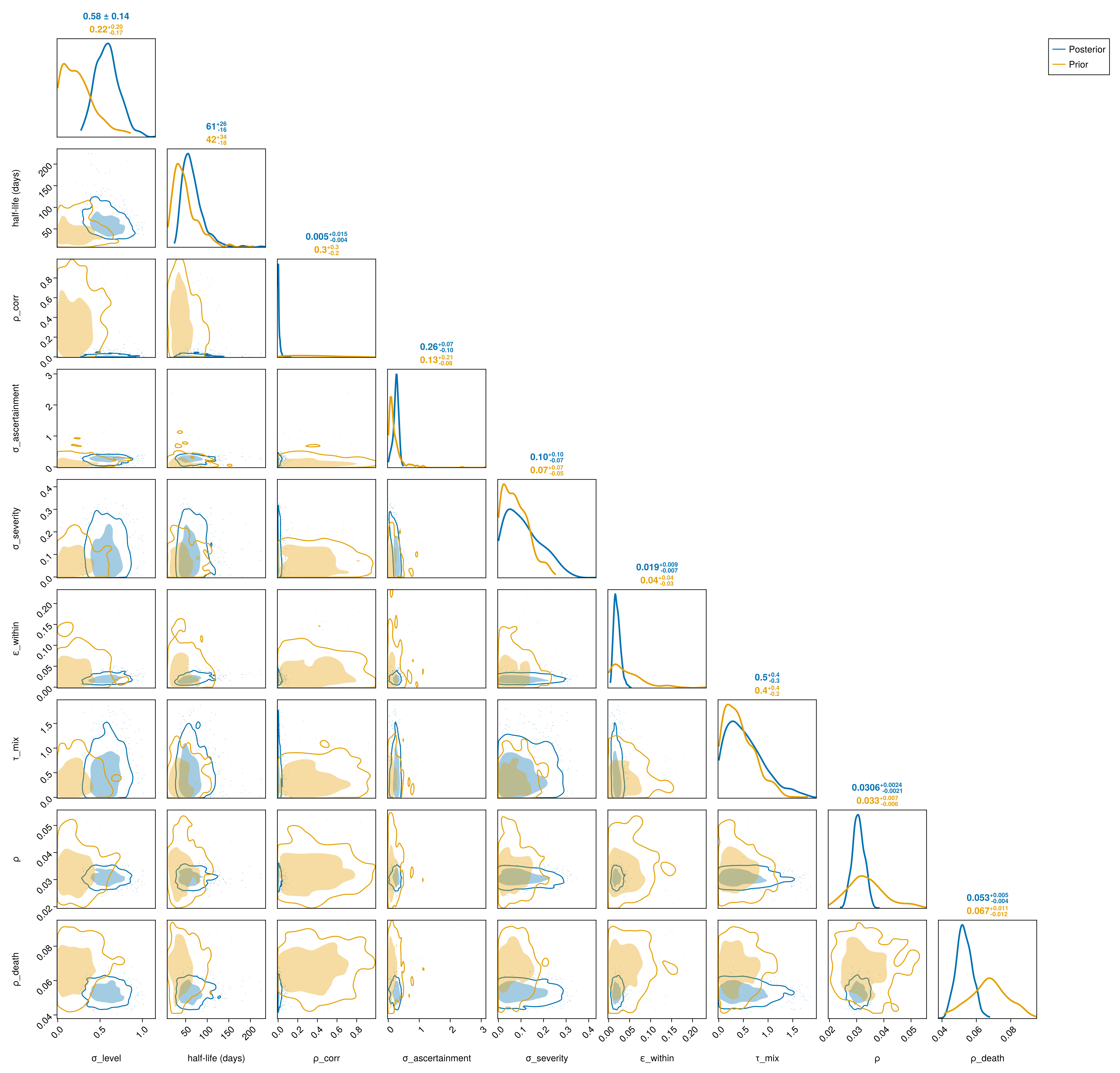
The table sets the posterior of each zone hyperparameter against its prior, with the ratio of their standard deviations. A ratio near one says the zone data add little to the prior. A ratio above one says the posterior is wider than the prior, which happens when the data move a parameter into the prior's wider tail. The drift scale is one per patch. The pair plot overlays the prior on the posterior of the scalar hyperparameters.
Draw from the zone model's prior
prior_chn_zone = zone_prior_draws(zone_inputs);Compute the zone prior and posterior table
# Each scalar zone hyperparameter with its table label and pair-plot axis
# label, kept where both chains carry it: the mixing and correlation
# blocks are sampled only when their inputs are on.
zone_hyper = [
    h for h in (
            (:region_sd_zone, "Level spread σ_level", "σ_level"),
            (:region_halflife_zone, "Deviation half-life (days)", "half-life (days)"),
            (:correlation_reference_zone, "Correlation ρ_corr", "ρ_corr"),
            (
                :zone_ascertainment_sd, "Ascertainment spread σ_ascertainment",
                "σ_ascertainment",
            ),
            (:zone_severity_sd, "Severity spread σ_severity", "σ_severity"),
            (:mixing_within_zone, "Within-patch mixing ε_within", "ε_within"),
            (:mixing_departure_zone, "Mixing departure τ_mix", "τ_mix"),
            (:composition_rho_zone, "Case composition ρ", "ρ"),
            (:composition_rho_death_zone, "Death composition ρ_death", "ρ_death"),
        )
        if BVDOutbreakSize._has_key(chn_local, h[1]) &&
        BVDOutbreakSize._has_key(prior_chn_zone, h[1])
]
zone_hyper_keys = first.(zone_hyper)
_hyper_draws(chn, k) = Float64.(vec(collect(chn[k])))
_drift_draws(chn, p) = Float64[
    v[p] for v in vec(collect(chn[:region_drift_sd_zone]))
]
function _prior_posterior_row(label, post, prior)
    f(x) = string(round(x; sigdigits = 3))
    ci(v) = string(
        f(median(v)), " (", f(quantile(v, 0.05)), "–",
        f(quantile(v, 0.95)), ")"
    )
    return (
        parameter = label, posterior = ci(post), prior = ci(prior),
        sd_ratio = round(std(post) / std(prior); digits = 2),
    )
end
zone_prior_table = DataFrame(
    vcat(
        [
            _prior_posterior_row(
                label, _hyper_draws(chn_local, k),
                _hyper_draws(prior_chn_zone, k)
            )
                for (k, label, _) in zone_hyper
        ],
        [
            _prior_posterior_row(
                "Drift scale σ_δ ($(zone_inputs.patch_labels[p]))",
                _drift_draws(chn_local, p), _drift_draws(prior_chn_zone, p)
            )
                for p in eachindex(zone_inputs.patch_labels)
        ]
    )
);
# The pair plot's axes take the symbols alone.
zone_hyper_pair_fig = plot_pair(
    chn_local, zone_hyper_keys;
    prior = prior_chn_zone,
    labels = Dict(k => sym for (k, _, sym) in zone_hyper)
);| parameter | posterior | prior | sd_ratio |
|---|---|---|---|
| Level spread σ_level | 0.575 (0.369–0.826) | 0.216 (0.0189–0.59) | 0.79 |
| Deviation half-life (days) | 60.9 (36.6–114.0) | 42.2 (14.6–106.0) | 0.88 |
| Correlation ρ_corr | 0.00518 (0.000286–0.0383) | 0.347 (0.0358–0.876) | 0.06 |
| Ascertainment spread σ_ascertainment | 0.257 (0.0692–0.381) | 0.126 (0.0252–0.669) | 0.3 |
| Severity spread σ_severity | 0.0988 (0.0092–0.256) | 0.069 (0.00693–0.182) | 1.39 |
| Within-patch mixing ε_within | 0.0188 (0.00859–0.035) | 0.0326 (0.00232–0.136) | 0.19 |
| Mixing departure τ_mix | 0.48 (0.0367–1.31) | 0.366 (0.0309–1.01) | 1.26 |
| Case composition ρ | 0.0308 (0.0271–0.0345) | 0.0329 (0.023–0.0457) | 0.33 |
| Death composition ρ_death | 0.0528 (0.0457–0.0607) | 0.067 (0.0493–0.0873) | 0.39 |
| Drift scale σ_δ (Ituri) | 0.244 (0.182–0.319) | 0.118 (0.067–0.211) | 0.93 |
| Drift scale σ_δ (Nord-Kivu) | 0.229 (0.162–0.338) | 0.122 (0.071–0.218) | 1.2 |
| Drift scale σ_δ (Haut-Uele) | 0.209 (0.133–0.318) | 0.122 (0.0684–0.215) | 1.24 |
| Drift scale σ_δ (Other provinces) | 0.122 (0.0692–0.22) | 0.12 (0.0663–0.221) | 0.97 |
Zone hyperparameter pair plot (prior overlaid)
Change over the past week
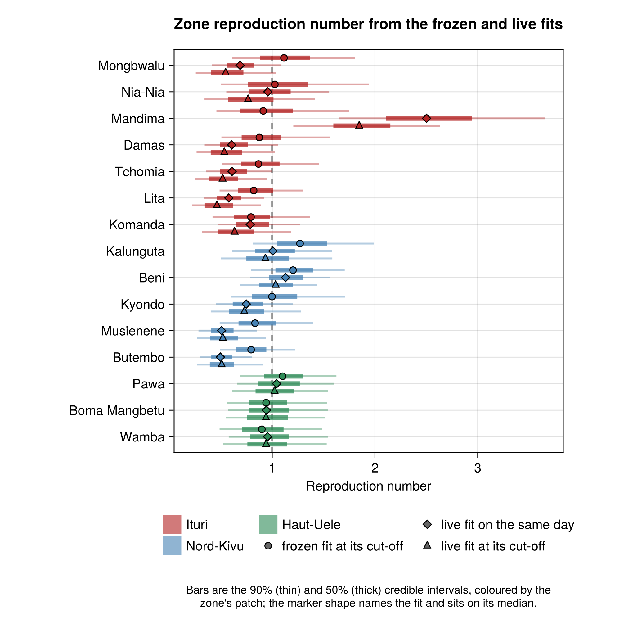
The health-zone model is melded onto the headline fit's patch infections one way, so the zone data do not update the national and province estimates. The comparison below reads the reproduction number of every zone walking in both fits at the frozen and live cut-offs, matched by key. The dot plot shows the fifteen zones the frozen fit ranks highest, the trajectories the twelve with most confirmed cases, and the table the ten with most confirmed cases.
Zone cut-off summaries shared by the comparisons
# One row per zone in `zs` with the median and the 50% and 90% intervals
# of its draws (one vector per zone), in the schema the zone dot plots
# read, plus the zone's key to match variants by and its confirmed cases
# to rank by. A zone with no finite draw is left out.
function _zone_cutoff_summary(draws, inputs, zs = eachindex(draws))
    keep = [i for (i, v) in enumerate(draws) if any(isfinite, v)]
    z = zs[keep]
    tbl = zone_summary_table(
        [filter(isfinite, draws[i]) for i in keep],
        inputs.zone_labels[z], inputs.patch_of_zone[z]
    )
    tbl.key = inputs.zone_keys[z]
    tbl.cases = inputs.cumulative[z]
    return tbl
end

# The `top` zones by confirmed cases in the first variant, one column per
# variant for the reproduction number. Each cell is a median with its 90%
# interval. Variants are matched by zone key.
function _zone_comparison_table(variants; top::Integer = 10)
    function cell(t, key, d, scale)
        i = findfirst(==(key), t.key)
        i === nothing && return ""
        f(x) = string(round(scale * x; digits = d))
        return string(f(t.median[i]), " (", f(t.lo90[i]), "–", f(t.hi90[i]), ")")
    end
    base = first(last(first(variants)))
    order = sortperm(base.cases; rev = true)[1:min(top, size(base, 1))]
    df = DataFrame(
        "Zone" => base.label[order],
        "Province" => [PROVINCE_LABELS[p] for p in base.patch[order]],
        "Cases" => base.cases[order]
    )
    for (q, name, d, scale) in ((:R, "R", 2, 1),),
            (label, s) in variants

        haskey(s, q) || continue
        df[!, "$name ($label)"] = [
            cell(s[q], k, d, scale)
                for k in base.key[order]
        ]
    end
    return df
end
_zone_comparison_table (generic function with 1 method)The frozen zone fit and the live one condition on different weeks of data and on different parent fits. The comparison reads each zone's reproduction number on the frozen cut-off day from both fits, alongside the live estimate at the current cut-off. A zone carries its own walk only once it has reported 30 confirmed cases, and the comparison is restricted to zones walking in both fits. The trajectory panels draw the frozen fit behind the live one for the twelve such zones with most confirmed cases.
Zone reproduction numbers from the frozen and live fits
# Daily reproduction numbers rebuilt from both fits, and the zones walking
# in both as live index => frozen index, matched by key. The summaries
# take their labels and cases from the live inputs.
zone_rt_live = reconstruct_zone_rt(chn_local, zone_inputs)
zone_rt_frozen = reconstruct_zone_rt(frozen_local.chn, frozen_zone_inputs)
zone_week_pairs = [
    z => j
        for (z, k) in enumerate(zone_inputs.zone_keys)
        for j in (findfirst(==(k), frozen_zone_inputs.zone_keys),)
        if j !== nothing && zone_inputs.walking[z] &&
        frozen_zone_inputs.walking[j]
]
zone_week_variants = let zs = first.(zone_week_pairs), js = last.(zone_week_pairs),
        n_f = frozen_zone_inputs.n

    [
        "frozen fit at its cut-off" => (;
            R = _zone_cutoff_summary(
                [zone_rt_frozen[j][:, n_f] for j in js],
                zone_inputs, zs
            ),
        ),
        "live fit on the same day" => (;
            R = _zone_cutoff_summary(
                [zone_rt_live[z][:, n_f] for z in zs],
                zone_inputs, zs
            ),
        ),
        "live fit at its cut-off" => (;
            R = _zone_cutoff_summary(
                [zone_rt_live[z][:, end] for z in zs],
                zone_inputs, zs
            ),
        ),
    ]
end
zone_week_table = _zone_comparison_table(zone_week_variants);
zone_week_fig = plot_zone_comparison(
    [l => s.R for (l, s) in zone_week_variants];
    xlabel = "Reproduction number", reference_line = 1.0,
    title = "Zone reproduction number from the frozen and live fits"
);

# The frozen trajectories padded onto the live grid, undefined past the
# frozen cut-off, behind the live ones over the zone grid. The plot reads
# an undefined day as `missing`, where the reconstruction writes `NaN`.
zone_week_rt_fig = let grid = zone_inputs.t0:obs.n, n_f = frozen_zone_inputs.n
    asmissing(m) = replace(m, NaN => missing)
    frozen = map(zone_week_pairs) do (z, j)
        m = fill(NaN, size(zone_rt_frozen[j], 1), obs.n)
        m[:, 1:n_f] .= zone_rt_frozen[j]
        asmissing(m[:, grid])
    end
    zs = first.(zone_week_pairs)
    plot_rt_zones(
        [asmissing(zone_rt_live[z][:, grid]) for z in zs],
        zone_inputs.zone_labels[zs], zone_inputs.patch_of_zone[zs];
        patch_labels = zone_inputs.patch_labels,
        dates = grid_date.(grid), as_of_date = obs.cutoff,
        cumulative = zone_inputs.cumulative[zs], top = 12,
        reference_rt = frozen, reference_label = "Frozen fit",
        title = "Zone reproduction number from the live fit, " *
            "with the frozen fit behind"
    )
end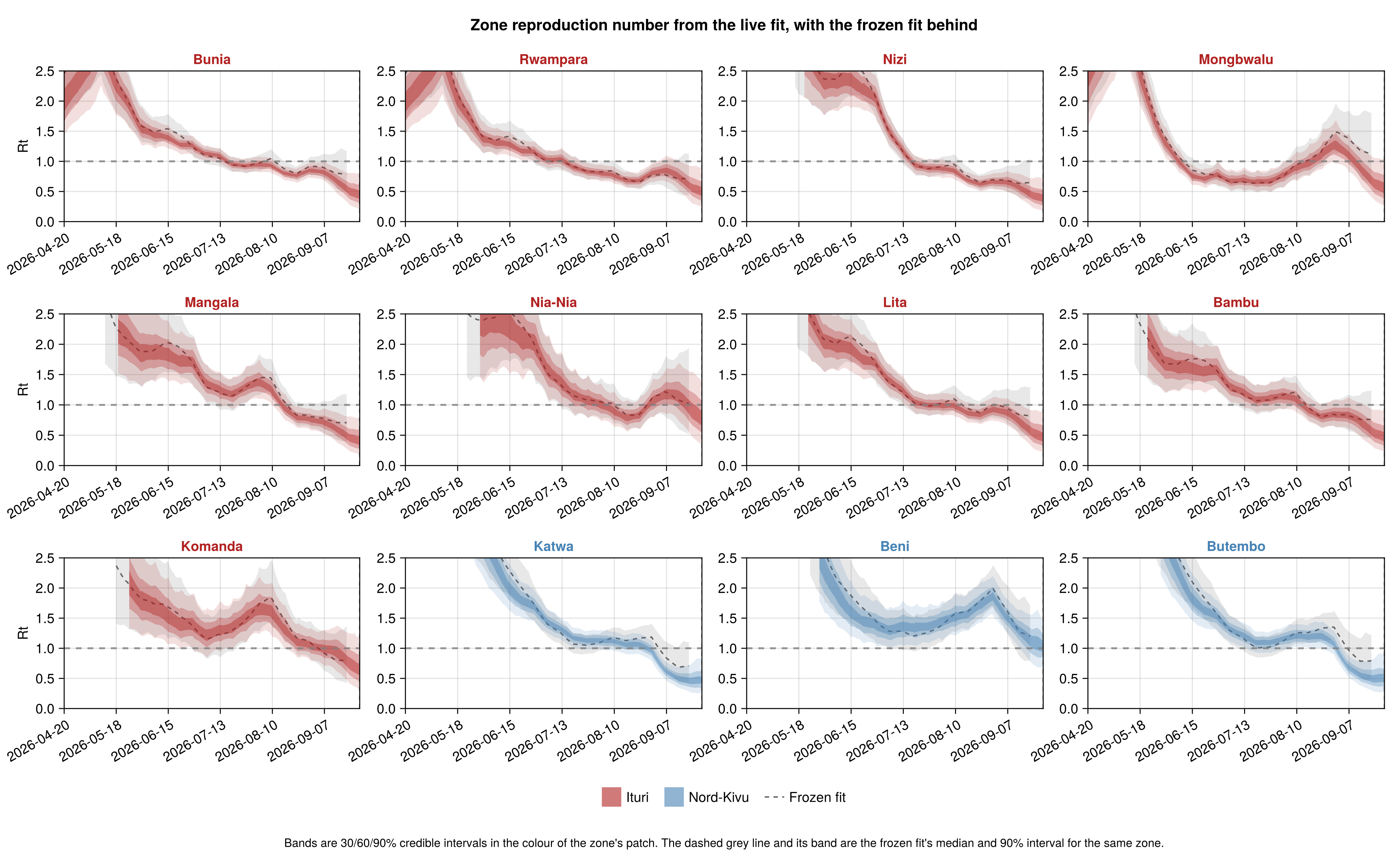
| Zone | Province | Cases | R (frozen fit at its cut-off) | R (live fit on the same day) | R (live fit at its cut-off) |
|---|---|---|---|---|---|
| Bunia | Ituri | 1697 | 0.79 (0.49–1.18) | 0.54 (0.33–0.81) | 0.44 (0.2–0.8) |
| Rwampara | Ituri | 1078 | 0.71 (0.43–1.13) | 0.6 (0.36–0.93) | 0.5 (0.24–0.9) |
| Nizi | Ituri | 771 | 0.64 (0.38–1.04) | 0.46 (0.27–0.72) | 0.38 (0.17–0.74) |
| Mongbwalu | Ituri | 697 | 1.12 (0.61–1.81) | 0.69 (0.41–1.09) | 0.55 (0.26–1.04) |
| Katwa | Nord-Kivu | 555 | 0.71 (0.44–1.1) | 0.46 (0.28–0.72) | 0.48 (0.26–0.84) |
| Mangala | Ituri | 346 | 0.71 (0.39–1.18) | 0.49 (0.28–0.81) | 0.4 (0.18–0.79) |
| Beni | Nord-Kivu | 329 | 1.2 (0.79–1.71) | 1.13 (0.79–1.56) | 1.03 (0.69–1.44) |
| Nia-Nia | Ituri | 284 | 1.03 (0.5–1.94) | 0.96 (0.55–1.56) | 0.77 (0.34–1.41) |
| Lita | Ituri | 283 | 0.82 (0.49–1.3) | 0.58 (0.34–0.92) | 0.46 (0.22–0.89) |
| Butembo | Nord-Kivu | 256 | 0.8 (0.49–1.22) | 0.5 (0.3–0.81) | 0.51 (0.27–0.91) |
Health-zone map
Each affected health zone coloured by its current reproduction number, with the chance that number exceeds one, the seven-day confirmed-case forecast, the chance of at least a chosen number of cases, the confirmed cases to date and the zone's share of its patch's infections available from the switcher. A filter shows the zones with or without a case over the past one, two or four weeks, and the reproduction number and the forecast can be read at their median or at either bound of the 90% interval. A zone whose reproduction number is from its province, not modelled separately, is hatched, and a filter shows either kind alone. A reproduction number whose 90% interval spans one is paler, and province outlines are drawn over the zones. Hover over a zone for its estimate and 90% credible interval, click it for every number, or open the table view to sort by any column. The map header gives the data cut-off and a link to download the estimates as a CSV file. The map needs a browser. It appears only on the documentation site.
Saving zone assets
The interactive map above reads the per-zone estimates written here. The zone forecast figure is written by the health-zone forecasts page and the frozen zone forecast and its scores by the health-zone forecast evaluation page.
Write the zone dashboard and release assets
dashboard_dir = joinpath(
    pkgdir(BVDOutbreakSize), "docs", "src", "summary_assets"
)
mkpath(dashboard_dir)
# The health-zone maps and the one-week zone forecast for the summary
# dashboard, and the per-zone estimates the interactive map reads: one row per zone keyed as the
# geojson keys it, with the cases and deaths to date, the reproduction
# number and the chance it exceeds one, the one-week forecast and the
# share of the patch's infections, whether the zone's reproduction number
# is modelled separately (`walking`) and the data cut-off. A zone below the
# reporting floor carries no reproduction number.
CairoMakie.save(joinpath(dashboard_dir, "zone_rt_map.png"), zone_map_fig)
_zone_deaths = [
    let h = obs.zone_death_history
        haskey(h, prov) && haskey(h[prov], z) &&
            !isempty(h[prov][z].counts) ? Int(h[prov][z].counts[end]) :
            0
    end
        for (prov, z) in zip(
            zone_inputs.zone_province,
            zone_inputs.zone_names
        )
]
_zone_rt_stat(f) = [isempty(r) ? missing : f(r) for r in zone_RT_finite]
zone_estimates = DataFrame(
    zone = zone_map_keys,
    label = zone_inputs.zone_labels, province = zone_inputs.zone_province,
    patch = zone_inputs.patch_labels[zone_patch],
    cases = zone_inputs.cumulative, deaths = _zone_deaths,
    R_T_median = _zone_rt_stat(median),
    p_rt_above_one = [
        isempty(r) ? missing : mean(r .> 1) for r in zone_RT_finite
    ],
    R_T_lower = _zone_rt_stat(r -> quantile(r, 0.05)),
    R_T_upper = _zone_rt_stat(r -> quantile(r, 0.95)),
    forecast_median = [median(v) for v in zone_fc_draws.zones],
    forecast_lower = [quantile(v, 0.05) for v in zone_fc_draws.zones],
    forecast_upper = [quantile(v, 0.95) for v in zone_fc_draws.zones],
    share_median = [median(v) for v in zone_share_T],
    share_lower = [quantile(v, 0.05) for v in zone_share_T],
    share_upper = [quantile(v, 0.95) for v in zone_share_T],
    p_ge_1 = zone_fc_probs[:, 1], p_ge_5 = zone_fc_probs[:, 2],
    p_ge_10 = zone_fc_probs[:, 3], p_ge_20 = zone_fc_probs[:, 4],
    cases_last_7 = zone_recent[7], cases_last_14 = zone_recent[14],
    cases_last_28 = zone_recent[28],
    last_case_date = [ismissing(d) ? "" : string(d) for d in zone_last_case],
    walking = Int.(zone_inputs.walking),
    as_of = fill(string(obs.cutoff), length(zone_map_keys))
)
CSV.write(joinpath(dashboard_dir, "zone_estimates.csv"), zone_estimates)
# The same frame into the release outputs.
output_dir = get(
    ENV, "BVD_OUTPUT_DIR",
    joinpath(pkgdir(BVDOutbreakSize), "output")
)
mkpath(output_dir)
CSV.write(joinpath(output_dir, "zone_estimates.csv"), zone_estimates)"/home/runner/work/BVDOutbreakSize/BVDOutbreakSize/output/zone_estimates.csv"The full analysis code, data and model definitions are in the epiforecasts/BVDOutbreakSize repository.