Methods

The data the estimates are built from, the model fitted to them, and how it is fitted and evaluated. The estimates themselves are on the other pages.

This page is generated from docs/pages/methods.jl. The model code it describes is in src/. See aim and origins and limitations.

Load packages, data and fitted chains

# Shared setup: packages, observations and the fit registry. See
# `docs/pages/_setup.jl`.
using BVDOutbreakSize
include(joinpath(pkgdir(BVDOutbreakSize), "docs", "pages", "_setup.jl"))

validation_forecast_from (generic function with 1 method)

Data

The DRC data come from the situation reports of the Institut National de Santé Publique (INSP, 2026). Each report gives the national cumulative suspected cases and deaths, laboratory-confirmed cases and deaths, and the specimens received and analysed by the laboratory, at the report date. From SitRep 013 (27 May) INSP began reclassifying suspects, so the cumulative suspected count falls. We freeze it at its last stable vintage (26 May) and instead read the daily new-suspect count ("nouveaux cas suspects du jour") that the confirmed-based reports publish from 4 June. We fit it as a daily incidence where the cumulative series stops. The same reports print a daily new suspected-death count alongside it ("cas suspects du jour N (M deces)", from 7 June). We fit it the same way, where the cumulative suspected-death series stops. The confirmed-based reports also publish a daily "Patients en isolement" count, the number of patients (confirmed plus suspected) in an isolation/treatment bed at the end of the day. We fit it as the suspect inflow carried through a length-of-stay survival into a daily bed count. The fitted series runs from 1 June (SitRep 018), where the column is relabelled to the all-patients "Patients en isolement - hospitalisation". The narrower suspects-only count in SitReps 016-017 is a different quantity and is left out. The reports also print a cumulative "cumul guéris" total of confirmed cases recorded as recovered, from 6 June. We fit it as survivors among the modelled confirmed cases (a scaled confirmation-to-recovery convolution, the incidence analogue of the isolation prevalence stream). From 13 June the reports add a Tableau 6 patient-movement table for the treatment centres. We read its daily admissions, in-care deaths, rule-outs and absconded flows as four count streams feeding the same treatment-centre model. The same table breaks the occupancy into "dont confirmés (NC+AC)" and "dont suspects" sub-rows, two prevalence sub-stocks that sum to the total each day. We read these as two further census streams splitting the occupancy. We extracted these figures from the written situation-report PDFs (archived by INRB-UMIE (INRB-UMIE, 2026)) using a language model, with a second pass to re-read them, rather than the published per-zone CSVs. The zone sums in the CSVs are inconsistent with the national headline totals because they drop counts not yet attributed to a zone, so they understate the national totals. The Uganda data are the cases and the one death exported across the border, taken from the WHO situation reports and Disease Outbreak News (World Health Organization, 2026). The cross-border traveller volume and source population come from McCabe and others (2026). The source population is fixed, and the traveller volume is given a Normal prior around the McCabe et al. figure. Province populations are 2019 figures from the DRC's Institut National de la Statistique, Annuaire statistique RDC 2020 (March 2021), as tabulated on the Wikipedia page for the provinces of the DRC (accessed 15 September 2026). Their relative sizes set the importation kernel and centre the background share, and their absolute sizes are the susceptible pools the renewal depletes. The distances in the importation kernel are between provincial population centres, the mean of each province's health-zone centroids weighted by WorldPop population (WorldPop, 2025), from the INRB-UMIE health-zone map (INRB-UMIE, 2026).

From SitRep 059 (12 July) the analytique-format situation reports also carry a raster figure of confirmed cases by symptom-onset date, split alive/deceased ("courbe épidémique par date de début des symptômes"). It has no accompanying data table, so we digitise it directly from the figure. Digitisation introduces error into the resulting counts. See the symptom-onset reporting delay submodel below for how the model accounts for that error.

The first table lists each figure at the cut-off, or at the date reporting stopped for that stream. The second table gives the per-date history of each situation-report stream. The model fits the between-report increments of these series, so a single date reduces to the cut-off total.

Loading observations and building the data table

observations_table = DataFrame(
    field = [
        "exported_cases",
        "exports_deaths",
        "suspected_deaths",
        "suspected_cases",
        "confirmed_cases",
        "confirmed_deaths",
        "onset_curve_reported",
        "specimens_analysed",
        "treatment_admissions",
        "treatment_deaths",
        "treatment_ruleouts",
        "treatment_absconded",
        "genetic_tmrca_bound",
        "daily_outbound_travellers (prior mean)",
        "daily_outbound_travellers_sd (prior SD)",
        "source_population",
    ],
    date = [
        history_last_date(grid_date, (; days = obs.export_case_days)),
        history_last_date(grid_date, (; days = obs.export_death_days)),
        hist_last_date(obs.deaths_history),
        hist_last_date(obs.reported_history),
        hist_last_date(obs.confirmed_history),
        hist_last_date(obs.confirmed_deaths_history),
        history_last_date(
            grid_date, (; days = obs.onset_curve_history.report_days)
        ),
        hist_last_date(obs.lab_history),
        hist_last_date(obs.treatment_admissions_history),
        hist_last_date(obs.treatment_deaths_history),
        hist_last_date(obs.treatment_ruleout_history),
        hist_last_date(obs.treatment_absconded_history),
        grid_date(obs.n - obs.tmrca_days),
        missing,
        missing,
        missing,
    ],
    value = [
        obs.exported_cases,
        obs.exports_deaths,
        obs.total_deaths,
        obs.reported_cases,
        obs.confirmed_cases,
        obs.confirmed_deaths,
        obs.onset_curve_history.last_total,
        obs.tests_analysed,
        isempty(obs.treatment_admissions_history.counts) ? missing :
            obs.treatment_admissions_history.counts[end],
        isempty(obs.treatment_deaths_history.counts) ? missing :
            obs.treatment_deaths_history.counts[end],
        isempty(obs.treatment_ruleout_history.counts) ? missing :
            obs.treatment_ruleout_history.counts[end],
        isempty(obs.treatment_absconded_history.counts) ? missing :
            obs.treatment_absconded_history.counts[end],
        obs.tmrca_days,
        ITURI_DAILY_TRAVEL,
        ITURI_DAILY_TRAVEL_SD,
        ITURI_POPULATION,
    ]
);

field	date	value
exported_cases	2026-05-23	3
exports_deaths	2026-05-14	1
suspected_deaths	2026-05-26	246
suspected_cases	2026-05-26	1077
confirmed_cases	2026-09-26	8067
confirmed_deaths	2026-09-26	3901
onset_curve_reported	2026-09-24	6133
specimens_analysed	2026-05-28	755
treatment_admissions	2026-08-02	147
treatment_deaths	2026-08-02	22
treatment_ruleouts	2026-08-02	93
treatment_absconded	2026-08-02	2
genetic_tmrca_bound	2026-03-15	195
daily_outbound_travellers (prior mean)		1871
daily_outbound_travellers_sd (prior SD)		200
source_population		4392200

The per-date cumulative history of the DRC situation-report streams, the national totals at each report date. Each stream's source is recorded alongside the observation data itself. Two columns are the exception. The new-suspect column is a per-day count, not a cumulative total, fitted directly as a daily incidence. It picks up where the cumulative suspected-case column freezes on 26 May. The isolated-patients column is a daily count of patients in an isolation/treatment bed, fitted as the suspect inflow carried through a length-of-stay survival.

Building the per-date time-series table

vintage_table = let
    # Each history carries grid day-indices and counts; key the counts
    # by calendar date so every stream lines up in one table.
    bydate(h) = Dict(grid_date(d) => c for (d, c) in zip(h.days, h.counts))
    streams = (
        suspected_cases = bydate(obs.reported_history),
        suspected_new_daily = bydate(obs.suspected_daily_history),
        patients_isolated = bydate(obs.isolation_history),
        suspected_deaths = bydate(obs.deaths_history),
        suspected_new_daily_deaths = bydate(obs.suspected_daily_deaths_history),
        confirmed_cases = bydate(obs.confirmed_history),
        confirmed_deaths = bydate(obs.confirmed_deaths_history),
        recovered_confirmed = bydate(obs.recovered_history),
        specimens_received = bydate(obs.tests_received_history),
        specimens_analysed = bydate(obs.lab_history),
    )
    dates = sort(collect(union((keys(s) for s in streams)...)))
    at(s) = [haskey(s, d) ? s[d] : missing for d in dates]
    DataFrame(
        date = dates,
        suspected_cases = at(streams.suspected_cases),
        suspected_new_daily = at(streams.suspected_new_daily),
        patients_isolated = at(streams.patients_isolated),
        suspected_deaths = at(streams.suspected_deaths),
        confirmed_cases = at(streams.confirmed_cases),
        confirmed_deaths = at(streams.confirmed_deaths),
        recovered_confirmed = at(streams.recovered_confirmed),
        specimens_received = at(streams.specimens_received),
        specimens_analysed = at(streams.specimens_analysed)
    )
end;

Per-date situation-report data table

date	suspected_cases	suspected_new_daily	patients_isolated	suspected_deaths	confirmed_cases	confirmed_deaths	recovered_confirmed	specimens_received	specimens_analysed
2026-05-14					8	4
2026-05-17					13	4
2026-05-18	516			131	33	4
2026-05-19	575			148	51	4
2026-05-20	672			160	64	6
2026-05-21	745			175	83	9
2026-05-22	872			204	91	10
2026-05-23	904			220	101	10		418	211
2026-05-24	906			223	105	10		431	295
2026-05-25	998			238	106	12		431	295
2026-05-26	1077			246	121	17		662	403
2026-05-27					125	17		774	648
2026-05-28					210	17		883	755
2026-05-29					263	42
2026-05-30					282	42
2026-05-31					321	48
2026-06-01			173		344	60
2026-06-02			206		363	62
2026-06-03			233		381	64
2026-06-04		153	258		452	82
2026-06-05		119	267		488	86
2026-06-06		117	283		515	91	12
2026-06-07		94	309		550	101	19
2026-06-08		138	297		598	115	22
2026-06-09		119	260		635	127	30
2026-06-10		119	262		676	136	32
2026-06-11		168	315		689	139	32
2026-06-13		136	359		782	181	40
2026-06-14		165	363		808	192	48
2026-06-15		235	376		837	196	49
2026-06-16		192	379		875	202	67
2026-06-17		151	383		896	232	78
2026-06-18		238	416		933	245	80
2026-06-19		162	361		956	247	92
2026-06-20		201	365		1003	254	100
2026-06-21		202	371		1048	267	112
2026-06-22		131	387		1094	277	115
2026-06-23		138	408		1118	291	122
2026-06-24		154	385		1155	304	138
2026-06-25		265	419		1203	321	148
2026-06-27		239	502		1274	360	178
2026-06-29		309	609		1333	399	189
2026-06-30		301			1406	438	208
2026-07-01		150	641		1460	452	213
2026-07-02		213	628		1502	473	229
2026-07-03		185			1528	492	239
2026-07-04		354			1561	506	254
2026-07-05		135	646		1624	521	273
2026-07-06		237	680		1708	580	280
2026-07-07		304	750		1759	600	285
2026-07-08		227	764		1792	625	295
2026-07-09		284	780		1830	648	300
2026-07-10		299	763		1873	672	306
2026-07-11		299	753		1926	702	318
2026-07-12		268	736		1963	719	333
2026-07-13		268	753		2011	754	366
2026-07-14		418	736		2073	796	377
2026-07-15		389	725		2124	828	390
2026-07-17		236	722		2267	893	412
2026-07-18		192	724		2344	930	466
2026-07-19		252	734		2423	967	469
2026-07-20		322	737		2473	999	482
2026-07-21		306	738		2536	1033	506
2026-07-22		318	722		2905	1269	519
2026-07-23		315	766		2973	1309	540
2026-07-24		274	755		3075	1354	556
2026-07-25		340	773		3200	1405	571
2026-07-26		326	723		3262	1437	583
2026-07-27		321	733		3360	1487	597
2026-07-30		374	748		3605	1587	651
2026-07-31		321	760		3674	1621	666
2026-08-01		227	690		3748	1657	708
2026-08-02		275	707		3802	1707	727
2026-08-03		289	717		3874	1751	749
2026-08-04		267	674		3973	1801	776
2026-08-05		282	694		4053	1851	793
2026-08-06			721		4120	1887	810
2026-08-07		443			4209	1916	828
2026-08-08		258	722		4294	1960	849
2026-08-09		242	704		4381	2011	869
2026-08-10		389	716		4449	2061	886
2026-08-11		325	570		4567	2128	918
2026-08-12		328	634		4665	2184	965
2026-08-13		330	749		4727	2214	976
2026-08-14		403	777		4843	2272	1006
2026-08-15		380	730		4945	2325	1040
2026-08-16		272	751		5021	2378	1061
2026-08-17		394	782		5105	2420	1091
2026-08-18		389	730		5208	2476	1115
2026-08-19		366	837		5290	2516	1152
2026-08-20		301	737		5375	2557	1167
2026-08-21		345	798		5458	2606	1182
2026-08-22		212	808		5514	2642	1200
2026-08-23		277	846		5584	2680	1215
2026-08-24		311	792		5656	2715	1245
2026-08-25		390	770		5713	2744	1269
2026-08-26		431	843		5794	2786	1293
2026-08-27		400	795		5863	2824	1318
2026-08-28		395	896		5945	2862	1327
2026-08-29		320			6041	2911	1366
2026-08-30		258	814		6100	2950	1383
2026-08-31		454	830		6186	3007	1409
2026-09-01		348	869		6250	3039	1439
2026-09-02		433	770		6342	3072	1475
2026-09-03		345	738		6436	3095	1495
2026-09-04		399	817		6522	3134	1516
2026-09-05		286	851		6604	3175	1548
2026-09-06		215	819		6686	3226	1563
2026-09-07		329	813		6757	3267	1590
2026-09-08		408	833		6843	3310	1611
2026-09-09		386	823		6942	3349	1647
2026-09-10		429	837		7022	3398	1671
2026-09-11		372	855		7113	3437	1692
2026-09-12		445	923		7200	3475	1712
2026-09-13		351	905		7258	3510	1726
2026-09-14		413	938		7345	3545	1753
2026-09-15		423	930		7404	3577	1776
2026-09-16		417	905		7475	3605	1798
2026-09-17		1329	930		7541	3639	1823
2026-09-18		360	909		7614	3676	1864
2026-09-19		427	886		7672	3699	1879
2026-09-20		318	821		7733	3732	1902
2026-09-21		359	839		7773	3759	1935
2026-09-22		449	885		7820	3779	1951
2026-09-23		353	893		7890	3799	1966
2026-09-24		300	848		7946	3833	2001
2026-09-25		321	828		7989	3852	2033
2026-09-26		355	773		8067	3901	2070

Model

Model overview

We model a single outbreak seeded by a zoonotic introduction on a daily grid from a seeding date to the cut-off (day ). The country is split into four patches, one each for Ituri, Nord-Kivu and Haut-Uele and a fourth pooling Sud-Kivu, Tshopo, Bas-Uele and Sud Ubangi. Each patch runs its own discrete renewal equation at its own reproduction number, and the patches are coupled by importation. National infection incidence is the sum over the patches. Every national stream is fitted against that sum. The patch reproduction numbers share one weekly trend and deviate from it, so a province with little data stays near the trend and one with data can separate from it. The situation reports' per-province tables are exact partitions of the national totals, so they enter as composition likelihoods carrying the spatial split alone. Setting the patch count to one collapses the model onto a single well-mixed population.

We never observe infections directly. Each data stream observes a thinned, delayed or transformed view of the same latent incidence. This is the class of time-varying renewal model used in EpiNow2 (Abbott et al., 2020), with the streams fitted jointly here rather than in a pipeline.

The model is assembled from modular Turing (Ge et al., 2018) submodels, each holding the maths and priors for one part of the generative process. We describe them in generative order, from the infection process through the epidemiological delays to the observation streams. The implementation uses Mooncake (Tebbutt and Ge, 2024) reverse-mode automatic differentiation, CensoredDistributions for delay discretisation, FlexiChains for chain handling, and PairPlots (Thompson, 2024) with AlgebraOfGraphics (Danisch and Krumbiegel, 2021) for the figures. Each submodel's source is shown in the collapsible block beneath its prose.

The table below shows which parameters inform each observation submodel. The analysed column is the analysed-specimen volume, the single laboratory stream fitted as a count. The confirmed positives are scored as a Binomial of the observed analysed denominator with a positivity linked to the composition of the suspected pool, so the laboratory data help identify the non-BVD background. The conf. deaths column mirrors the laboratory pipeline on the death side, with a death testing intensity and a death-pool composition positivity built from the same assay:

Parameter	Exports	Deaths	Cases	Analysed	Confirmed	Conf. deaths	Export deaths
Reproduction number	●	●	●	●	●	●	●
Generation interval	●	●	●	●	●	●	●
Incubation period	●	●	●	●	●	●	●
Cryptic-phase seed	●	●	●	●	●	●	●
Onset-to-death delay		●				●	●
Case-fatality ratio		●				●	●
Death ascertainment		●				●
Background CFR		●				●
Onset-to-report delay			●	●	●
Receipt delay				●	●	●
Onset-to-hospitalisation delay	●
Assay sensitivity / specificity					●	●
Severity enrichment					●
Death testing intensity						●
Testing fraction				●	●
Background rate		●	●	●	●	●
Surveillance dispersion		●	●	●
Ascertainment	●		●	●	●		●
Traveller volume	●						●

Infections

Reproduction number

Each patch has its own daily reproduction number. It is a shared trend plus a patch deviation , with the deviations summing to zero across patches on every day:

The country's reproduction number is read off the summed infections in the infection process below.

The trend is held flat at the established reproduction number until a month before the first WHO situation report. It then follows a non-centred Gaussian random walk on the log scale with weekly knots to the cut-off. The walk start is floored at the renewal start. The walk starts from at its first knot:

We do not place a prior on directly. We put the prior on the initial growth rate instead, given in the seeding and growth subsection below, and derive the established reproduction number forward from it through the Euler–Lotka relation under our generation interval :

We set the half-normal on so that the trend is unlikely to change by more than about 20% from one week to the next: two standard deviations of the weekly log-step is around .

Daily is the linear interpolation between the weekly knots. Before the first knot it is held flat at (the interpolation clamps below the first knot rather than extrapolating):

with the day of knot . The outbreak response adds a sampled effect shaped by a logistic ramp at the first WHO situation report on 18 May 2026. We assume the response takes about three weeks (21 days) to take effect, and that it can only reduce transmission. The effect is therefore constrained to be non-positive:

The deviations live on the trend's weekly knots  . They are correlated across patches, they revert toward zero, and they sum to zero at every knot so that no patch is privileged. A sum-to-zero vector over patches has   free directions, so the deviations are drawn on them through a fixed orthonormal basis (  , columns orthogonal to the vector of ones):

with  , the lower-triangular Bartlett factor of the Wishart draw (Bartlett, 1934; Smith and Hocking, 1972) and   the per-knot retention set by , the half-life in days of a patch's divergence from the trend. is a Helmert basis, the isometric log-ratio basis of compositional data analysis (Egozcue et al., 2003) that Stan uses for its sum-to-zero vector (Carpenter et al., 2017; Stan Development Team, 2026). sets the shape of the innovation covariance and its size, since the covariance has trace   whatever is. Together they are a full covariance of a sum-to-zero vector, and   gives every patch the trend's shape. Each knot draws   values, one per direction the deviations can move in. The Wishart prior does not change under a rotation of the basis, so every patch and every pair of patches has the same prior whatever order the patches come in. Each patch's innovation then has expected variance  , as it would with a scale   on independent patch innovations with their mean removed. We report the per-patch innovation standard deviations and their   correlation derived from it. The correlations of a sum-to-zero vector cannot all be positive, and with equal standard deviations each patch's correlations with the others average  . Daily is the interpolation of the knot series, as for the trend.

Submodel: patch_rt_model

@model function patch_rt_model(
        n::Integer, n_patches::Integer,
        log_R0_base::Real;
        breakpoint::Union{Missing, Real} = missing,
        week::Integer = 7,
        rt_start::Integer = 1,
        rt_walk_start::Integer = rt_start,
        rt = rt_walk_model,
        region_sd_prior = truncated(Normal(0, 0.15); lower = 0),
        region_drift_sd_prior = truncated(Normal(0, 0.05); lower = 0),
        region_halflife_prior = LogNormal(log(42), 0.6),
        region_offset_prior = Normal(0, 1),
        basis = sum_to_zero_basis(n_patches),
        forecast::Union{Nothing, ForecastHorizon} = nothing
    )
    ## Common national trend, the single-patch walk unchanged.
    ## `rt_walk_start` maps to `rt_start` in the inner model, matching the
    ## convention in [`infection_model`](@ref). Attached prefixed (no
    ## `false`), so the walk's parameters reach the chain as
    ## `rt_state.sigma_rw`, `rt_state.log_R0`, `rt_state.z` and
    ## `rt_state.intervention_effect`, the names the analysis and sensitivity
    ## pages read. Attaching it unprefixed surfaces them bare and fails at
    ## render time on a KeyError.
    fkw = forecast === nothing ? (;) : (; forecast)
    rt_state ~ to_submodel(
        rt(n, log_R0_base; breakpoint, rt_start = rt_walk_start, fkw...)
    )
    Rt_national = rt_state.Rt
    ## The deviations live on the same weekly knots as the national walk, so
    ## both processes are described at the same resolution.
    days = knot_days(n; week, start = rt_walk_start)
    nb = length(days)
    ## Grid length, past the cut-off when forecasting.
    ng = length(Rt_national)
    ## Single patch. The deviations are sum-to-zero across the patches, so
    ## with one patch delta is identically zero and the patch Rt is the
    ## national walk. Sampling the deviation machinery would then add
    ## prior-only dimensions the likelihood never touches, so it is skipped
    ## entirely and `n_patches = 1` collapses this model exactly onto the
    ## single-population one.
    if n_patches == 1
        Tp1 = eltype(Rt_national)
        δ_patch1 = zeros(Tp1, 1, ng)
        Rt_matrix1 = zeros(Tp1, 1, ng)
        @inbounds for t in 1:ng
            Rt_matrix1[1, t] = Rt_national[t]
        end
        return (;
            Rt_matrix = Rt_matrix1, Rt_national,
            δ_patch = δ_patch1, δ_knots = zeros(Tp1, 1, nb),
            σ_level = zero(Tp1), σ_δ = zeros(Tp1, 1),
            Ω = ones(Tp1, 1, 1), drift_factor = zeros(Tp1, 1, 0),
            δ_halflife = zero(Tp1),
            sigma_rw = rt_state.sigma_rw,
            log_R0 = rt_state.log_R0,
            intervention_effect = rt_state.intervention_effect,
        )
    end
    ## Mean reversion. The deviations are an AR(1) toward zero on the knots,
    ## parameterised by the half-life of a provincial divergence in days,
    ## which is the elicitable quantity. The per-knot retention is
    ## `phi = 2^(-week / halflife)`, so a half-life far longer than the
    ## window recovers the random walk and a short one pulls each province
    ## back to the national trend between knots. One half-life is shared
    ## across provinces, not one each: the retention multiplies the whole
    ## deviation vector, and a sum-to-zero vector scaled by a scalar still
    ## sums to zero.
    σ_level ~ region_sd_prior
    δ_halflife ~ region_halflife_prior
    φ = exp2(-week / δ_halflife)
    ## Loading matrices from the `n_patches - 1` sum-to-zero directions to
    ## the patches: a Bartlett factor of a Wishart covariance on the
    ## directions, whose prior treats every patch alike, gives the shape.
    ## The factor is rescaled to trace `n_patches - 1`, so `σ_drift` alone
    ## sets the size of the innovations and can shrink them to zero. With
    ## two patches there is one direction and no lower entry to draw.
    nd = n_patches - 1
    σ_drift ~ region_drift_sd_prior
    bartlett_diag ~ product_distribution([Chi(nd - j + 1) for j in 1:nd])
    if nd > 1
        bartlett_lower ~ product_distribution(
            fill(Normal(0, 1), nd * (nd - 1) ÷ 2)
        )
    else
        bartlett_lower = Float64[]
    end
    A = bartlett_factor(bartlett_diag, bartlett_lower)
    shape_scale = sqrt(nd / sum(abs2, A))
    F_drift = sum_to_zero_factor(basis, σ_drift * shape_scale, A)
    F_level = sum_to_zero_factor(basis, σ_level * shape_scale, A)
    ## Standard-normal draws for the level and for each knot's innovation,
    ## `n_patches - 1` per knot.
    z_level ~ product_distribution(fill(region_offset_prior, nd))
    z_drift ~ product_distribution(
        fill(region_offset_prior, max(nd * (nb - 1), 1))
    )
    Tp = promote_type(
        eltype(Rt_national), eltype(F_level), eltype(F_drift),
        eltype(z_level), eltype(z_drift), typeof(φ)
    )
    δ_knots = zeros(Tp, n_patches, nb)
    lvl = sum_to_zero(F_level, z_level)
    @inbounds for i in 1:n_patches
        δ_knots[i, 1] = lvl[i]
    end
    ## Every knot's innovation in one product, column `k - 1` for knot `k`,
    ## then the AR(1) retention as a scan over the knots.
    if nb > 1
        innovations = F_drift * reshape(z_drift, nd, nb - 1)
        @inbounds for k in 2:nb, i in 1:n_patches
            δ_knots[i, k] = φ * δ_knots[i, k - 1] + innovations[i, k - 1]
        end
    end
    ## Interpolate each patch's deviation to the daily grid and build Rt.
    ## Past the cut-off the deviations carry on reverting on knots a week
    ## apart, with fresh standard-normal draws `z_drift_future` through the
    ## same fitted loading, so the future innovations keep the fitted
    ## sum-to-zero correlation. The fitted knots are kept as they are.
    if forecast !== nothing
        fdays = future_knot_days(n, horizon_days(forecast); week)
        nf = length(fdays)
        z_drift_future ~ product_distribution(
            fill(region_offset_prior, nd * nf)
        )
        Tf = promote_type(Tp, eltype(z_drift_future))
        knots_all = zeros(Tf, n_patches, nb + nf)
        knots_all[:, 1:nb] .= δ_knots
        innovations_f = F_drift * reshape(z_drift_future, nd, nf)
        @inbounds for k in 1:nf, i in 1:n_patches
            knots_all[i, nb + k] = φ * knots_all[i, nb + k - 1] +
                innovations_f[i, k]
        end
        days_all = vcat(days, fdays)
    else
        knots_all = δ_knots
        days_all = days
    end
    Rt_matrix = zeros(eltype(knots_all), n_patches, ng)
    @inbounds for p in 1:n_patches
        ## A view, not a copy: `interpolate_knots` only reads its knots.
        δ_daily = interpolate_knots(view(knots_all, p, :), days_all, ng)
        for t in 1:ng
            Rt_matrix[p, t] = Rt_national[t] * exp(δ_daily[t])
        end
    end
    δ_patch = _detached(_daily_deviations, δ_knots, days, n)
    drift_moments = _detached(sum_to_zero_moments, F_drift)
    σ_δ = drift_moments.sd
    Ω = drift_moments.cor
    return (;
        Rt_matrix, Rt_national, δ_patch, δ_knots,
        σ_level, σ_δ, Ω, drift_factor = F_drift, δ_halflife,
        sigma_rw = rt_state.sigma_rw, log_R0 = rt_state.log_R0,
        intervention_effect = rt_state.intervention_effect,
    )
end

Submodel: rt_walk_model

@model function rt_walk_model(
        n::Integer, log_R0_base::Real;
        week::Integer = 7,
        breakpoint::Union{Missing, Real} = missing,
        rt_start::Integer = 1,
        ramp::Real = RT_INTERVENTION_RAMP,
        sigma_prior = truncated(Normal(0, 0.1); lower = 0),
        effect_prior = truncated(Normal(0, 0.4); upper = 0),
        forecast::Union{Nothing, ForecastHorizon} = nothing
    )
    days = knot_days(n; week, start = rt_start)
    nb = length(days)
    ## The established `R0` at the genetic bound is the base the walk grows
    ## from. It is derived and passed in, not sampled here, and tracked as a
    ## deterministic so it stays available on the chain.
    log_R0 := log_R0_base
    sigma_rw ~ sigma_prior
    z ~ product_distribution(fill(Normal(0, 1), max(nb - 1, 1)))
    intervention_effect ~ effect_prior
    steps = sigma_rw .* z[1:(nb - 1)]
    log_R = log_R0 .+ vcat(zero(log_R0), cumsum(steps))
    ## Past the cut-off the walk continues from its last fitted knot, one
    ## knot a week, with innovations of its own step size. They are a new
    ## variable, so the fitted knots and their density are untouched.
    ng = n + horizon_days(forecast)
    if forecast !== nothing
        fdays = future_knot_days(n, horizon_days(forecast); week)
        z_future ~ product_distribution(fill(Normal(0, 1), length(fdays)))
        log_R = vcat(log_R, log_R[end] .+ cumsum(sigma_rw .* z_future))
        days = vcat(days, fdays)
    end
    log_Rt = interpolate_knots(log_R, days, ng)
    log_Rt = log_Rt .+ intervention_effect .* sigmoid_ramp(ng, breakpoint; ramp)
    Rt = exp.(log_Rt)
    return (; Rt, log_R, days, sigma_rw, log_R0, intervention_effect)
end

Generation interval

We assume the generation interval is a Gamma distribution with a sampled mean and standard deviation . These are taken from the Ebola virus disease serial interval used as a generation-time proxy (fitted Gamma, mean 15.3 d, SD 9.3 d, from 92 transmission pairs; WHO Ebola Response Team 2014). The source reports no interval on either value, so each prior's spread is the sampling standard error of that estimate from 92 pairs,   d for the mean and about 1.0 d for the SD:

That puts 95% of the prior mean between 13.4 and 17.2 d and of the prior SD between 7.3 and 11.3 d. The Gamma shape and scale follow from them.

The Gamma is discretised through the same double-interval-censoring route as every delay, described with the first epidemiological process model below. That gives a probability mass function (PMF) , the probability assigned to each whole-day lag. The lag-0 bin is dropped and the remainder renormalised, so the generation interval starts at one day and an infectee is infected strictly after its infector.

Submodel: generation_interval_model

@model function generation_interval_model(
        nmax::Integer;
        mean_prior = truncated(Normal(15.3, 0.97); lower = 1),
        sd_prior = truncated(Normal(9.3, 1.0); lower = 1)
    )
    gi_mean ~ mean_prior
    gi_sd ~ sd_prior
    α = (gi_mean / gi_sd)^2
    θ = gi_sd^2 / gi_mean
    ## Unchecked, so a proposal that overflows `gi_mean` (as the step-size
    ## search at the start of warm-up can) gives a non-finite density the
    ## sampler rejects rather than a `DomainError` at `θ = 0`.
    dist = Gamma(α, θ; check_args = false)
    pmf = discretise_censored(dist, nmax)
    g = pmf[2:end] ./ sum(pmf[2:end])
    return (; g, gi_mean, gi_sd, gi_alpha = α, gi_theta = θ)
end

Seeding and growth

We assume the outbreak started from a zoonotic spillover and grew deterministically through an unobserved cryptic exponential phase lasting transmission generations before sustained transmission was established. The origin therefore sits    days before the renewal start, with the mean generation interval, and the cryptic phase grows one infection per day at the origin to   per day at the renewal start, the day the renewal takes over. Field epidemiology in Mongbwalu traced a sustained transmission chain back to a death on 25 January 2026, and identified more than 500 suspected cases between mid-January and mid-May (Kupferschmidt, 2026). The genetic TMRCA (Mbala-Kingebeni and others, 2026) is a lower bound on the outbreak age that is consistent with, but does not by itself fix, an origin that early. We place a prior on centred so that the implied origin sits in mid-February, with 90% of its mass between mid-January and mid-March:

The traced 25 January death then sits near the 87th percentile: it is the earliest chain the field work reached, which bounds the origin rather than dating it.

The growth rate carries the prior the genetic source informs. The BEAST X reanalysis of 139 BDBV genomes (Mbala-Kingebeni and others, 2026) reports an Exponential-growth doubling time of 11.7 d (95% HPD 6.8–17.5). We put a log-normal prior on equivalent to a log-normal prior on the doubling time centred on 11.7 d. Its log spread of 0.30 is a quarter wider than the 0.24 that HPD implies. The HPD is conditional on a single-rate coalescent, the assumption the field epidemiology above contradicts (Kupferschmidt, 2026). An earlier reanalysis of the first ten genomes, which the BEAST X rate supersedes, put the doubling time at 15.2–24.5 d (Cuomo-Dannenburg and Ghafari, 2026). Our 95% interval on the doubling time is 6.5–21.1 d, which contains the HPD and reaches into that earlier range:

This single growth rate fills the cryptic phase and, through the forward Euler–Lotka derivation above, sets the established reproduction number. The genetic report's own established reproduction number of about to uses its own generation interval.

The outbreak is assumed to have begun in Ituri, so the primary patch carries the whole cryptic seed and the others start empty:

with the renewal start. When a secondary patch first carries infections then follows from the kernel and the coupling intensity of the mixing subsection below.

Submodel: exponential_growth_model

@model function exponential_growth_model(
        g::AbstractVector;
        r_prior = LogNormal(log(log(2) / M_PRIOR_DOUBLING_DAYS), 0.3),
        m_prior = truncated(Normal(2.75, 1.2); lower = 0)
    )
    r ~ r_prior
    m ~ m_prior
    ## Mean generation interval, the unit `m` is counted in. `g` is indexed
    ## from one day, so the mean is `Σ i·g[i]`.
    G := sum(i * g[i] for i in eachindex(g))
    τ := log(2) / r
    ## Outbreak age is generations times the generation interval, so it does
    ## not depend on `r`.
    T := m * G
    ## Daily incidence at the renewal start, grown from one infection per day
    ## at the origin over `T` days at the cryptic rate.
    C_T := exp(r * T)
    return (; τ, r, m, T, C_T, G)
end

Genetic bound on outbreak age

A BEAST time tree of the first ten sequenced genomes (Amuri-Aziza et al., 2026) places the TMRCA, the age of the oldest internal node of the tree, at a mean of 25 March 2026. The temporal sampling range is too short to estimate the molecular clock, so we fix it to the   substitutions/site/year rate of the 2013-2016 West African Ebola epidemic (Holmes et al., 2016). The TMRCA is a lower bound on the outbreak age. Adding sequences, or more geographically representative ones, can only push the TMRCA earlier, never later. This is because the sampled tree is almost entirely from Bunia. Using the genetic TMRCA as a one-sided seeding bound rather than a point estimate follows a suggestion of Ferguson (2026).

We treat the TMRCA day as a right-censored, noisy reading of the total outbreak age (the cryptic duration plus the observed window, defined in the infection process below):

The renewal starts on the grid day on which the renewal recursion begins and sustained transmission is treated as established. We place it 14 days after the genetic TMRCA day, past the molecular-clock uncertainty, so the observed window from the renewal start to the cut-off is shorter than the TMRCA age. The bound therefore stays informative on the cryptic duration, pulling the origin to sit at or before the most recent common ancestor and bounding the cryptic phase from below. It is one-sided, leaving the age free above the TMRCA. We fix the clock and do not propagate cross-outbreak or clock uncertainty.

Submodel: genetic_seeding_model

@model function genetic_seeding_model(
        T::Real,
        tmrca_days::Union{Missing, Real}; tmrca_days_sd::Real = 16.0
    )
    if !ismissing(tmrca_days)
        tmrca_days ~ censored(Normal(T, tmrca_days_sd); upper = tmrca_days)
    end
    return (; T, tmrca_days_sd)
end

Mixing and importation

We model connectivity between provinces as a gravity kernel, proportional to destination population and inverse to the distance between provincial population centres. Each centre sits where the province's people live rather than at its capital. A pooled province takes the population-weighted mean of its members' centres. Each origin column is scaled so that the share of its transmission that leaves is the population share of the rest of the country,  :

The intensity is one level per origin, partially pooled, and it changes at detection on the logistic ramp the reproduction number uses:

with the fixed sum-to-zero basis of Equation (6), so the origin levels are centred on on the log scale. The origin deviation is drawn independently of the reproduction number deviations and is constant in time. Exports scale with through the origin's generated infections in Equation (18), and changes the share of them exported.

Submodel: province_importation_kernel

function province_importation_kernel(
        pops::AbstractVector = PROVINCE_POPULATIONS;
        distances::AbstractMatrix = province_distance_matrix(
            PROVINCE_CENTRES[1:min(length(pops), end)]
        ),
        decay::Real = PROVINCE_DISTANCE_DECAY
    )
    np = length(pops)
    size(distances) == (np, np) || error(
        "province_importation_kernel: `distances` is $(size(distances)) " *
            "but there are $np provinces."
    )
    tot = sum(pops)
    pull = gravity_pull(pops; distances, decay)
    K = zeros(Float64, np, np)
    @inbounds for q in 1:np
        s = sum(@view pull[:, q])
        s > 0 || continue
        ## Hold the column total at the pre-distance value, so the distance
        ## redistributes a province's exports without changing their volume.
        outflow = 1 - pops[q] / tot
        for p in 1:np
            K[p, q] = outflow * pull[p, q] / s
        end
    end
    return K
end

Infection process

The renewal start and observed window from the genetic bound above are

The grid days before the renewal start are filled by the cryptic exponential seeds above. This gives the recursion a full generation interval of history. Each patch then runs its own renewal forward at its own reproduction number, importation relocates a share of each day's new infections, and the result depletes the patch's susceptible pool:

This is the population adjustment of Bhatt et al. (2023), as used in EpiNow2 (Abbott et al., 2020), with the patch's resident population and starting at less the seeds. is the reproduction number in a fully susceptible population, and every reproduction number we report is net of depletion,  .

National infections are the patch sum, and the national reproduction number is read off that sum by inverting the renewal equation:

is what the headline reports. It sits above the trend , because the deviations are centred unweighted while the sum weights each patch by its share of the force, and the faster patch keeps gaining share.

Cumulative infections are the running sum of the daily national series. The cumulative infection count at the cut-off is the headline outbreak size. The total outbreak age is the cryptic duration plus the observed window:

The current growth rate is the exponential growth implied by the cut-off reproduction number and the generation interval through forward Euler–Lotka. The current doubling time is divided by that rate.

Submodel: patch_infection_model

@model function patch_infection_model(
        n::Integer, n_patches::Integer;
        breakpoint::Union{Missing, Real} = missing,
        rt_start::Integer = 1,
        rt_walk_start::Integer = rt_start,
        rt = patch_rt_model,
        gi = generation_interval_model,
        growth = exponential_growth_model,
        gi_nmax::Integer = cdf_nmax(Gamma(2.71, 5.65)),
        importation_kernel::AbstractMatrix = province_importation_kernel(
            PROVINCE_POPULATIONS[1:min(n_patches, end)]
        ),
        importation_epsilon_prior = Beta(1, 100),
        importation_sd_prior = truncated(Normal(0, 0.5); lower = 0),
        importation_effect_prior = Normal(0, 0.5),
        seed_fraction_prior = LogNormal(log(0.05), 1.0),
        basis = sum_to_zero_basis(n_patches),
        incubation = (nmax) -> censored_delay_model(
            nmax;
            mean_prior = truncated(Normal(6.3, 0.54); lower = 1),
            sd_prior = truncated(Normal(3.5, 0.8); lower = 1)
        ),
        incubation_nmax::Integer = cdf_nmax(lognormal_meansd(6.3, 3.5)),
        populations::AbstractVector{<:Real} = n_patches == 1 ?
            [float(sum(PROVINCE_POPULATIONS))] :
            float.(PROVINCE_POPULATIONS[1:n_patches]),
        forecast::Union{Nothing, ForecastHorizon} = nothing
    )
    ## Grid length, past the cut-off `n` when forecasting.
    ng = n + horizon_days(forecast)
    fkw = forecast === nothing ? (;) : (; forecast)
    ## 1. Shared generation interval.
    gi_state ~ to_submodel(gi(gi_nmax))
    g = gi_state.g
    ## 2. One growth source, as in [`infection_model`](@ref). The prior is on
    ##    the cryptic growth rate `r`, and the established `R0` (the walk
    ##    base) is derived forward from it through Euler-Lotka.
    growth_state ~ to_submodel(growth(g))
    r_clock = growth_state.r
    R0 = r_to_R0(r_clock, g)
    ## 3. Per-patch Rt: national trend plus per-patch deviations.
    rt_state ~ to_submodel(
        rt(
            n, n_patches, log(R0);
            breakpoint, rt_start, rt_walk_start, fkw...
        ), false
    )
    Rt_matrix = rt_state.Rt_matrix
    δ_patch = rt_state.δ_patch
    ## 4. Per-patch seeds. The primary patch takes the cryptic exponential.
    ##    Each secondary patch takes a fraction of that seed, which is the
    ##    scale the data speak to. With importation off the relative seed
    ##    sets the level of the provincial case split, leaving `δ_p` to be
    ##    identified by its time trend. An absolute seed prior pinned far
    ##    below the primary's `C_T` would force `δ_p` to absorb the whole
    ##    level difference, making the reported provincial Rt gap an artefact
    ##    of the seed prior.
    renewal_start = clamp(rt_start, 1, n)
    τ_obs = n - renewal_start
    seed0_total = seed_at_renewal_start(growth_state.C_T)
    ## The outbreak is assumed to have begun in Ituri, so the primary patch
    ## takes the whole cryptic seed and the others are seeded by importation
    ## from it. An
    ## all-zero kernel leaves a secondary patch no route to infections at
    ## all, so the uncoupled path keeps the sampled fractions. With one patch
    ## there is nothing to seed and the fraction would be a prior-only
    ## dimension either way.
    coupled = any(!iszero, importation_kernel)
    if n_patches > 1 && !coupled
        seed_fraction ~ product_distribution(
            fill(seed_fraction_prior, n_patches - 1)
        )
    else
        seed_fraction = Float64[]
    end
    Tp = promote_type(
        eltype(Rt_matrix), eltype(g), typeof(float(r_clock)),
        eltype(seed_fraction), typeof(float(seed0_total))
    )
    ## The fractions partition the national cryptic seed, they do not add to
    ## it. `growth_state.C_T` is `exp(r·m·G)` and the `m` prior is
    ## elicited as a national quantity, so it is the national daily
    ## incidence at the renewal start.
    ## Dividing through by `(1 + Σf)` keeps the national seed at `C_T` for any
    ## number of patches, so `C_T` stays comparable across `n_patches` and the
    ## genetic prior keeps its meaning.
    seed_shares = zeros(Tp, n_patches)
    if isempty(seed_fraction)
        seed_shares[1] = one(Tp)
    else
        seed_denom = one(Tp) + sum(seed_fraction)
        seed_shares[1] = one(Tp) / seed_denom
        @inbounds for p in 2:n_patches
            seed_shares[p] = seed_fraction[p - 1] / seed_denom
        end
    end
    seeds_matrix = zeros(Tp, n_patches, renewal_start)
    @inbounds for p in 1:n_patches
        ## A scaled copy of the same cryptic curve: each province is a share
        ## of one epidemic, so it grows at the same clock rate `r` over the
        ## cryptic window.
        s_p = seed_infections(
            seed_shares[p] * seed0_total, r_clock, renewal_start
        )
        for j in 1:renewal_start
            seeds_matrix[p, j] = s_p[j]
        end
    end
    ## 5. Importation intensity: one level per origin, partially pooled, and
    ##    a common change at detection on the ramp the reproduction number
    ##    already uses. Only sampled when the kernel couples the patches,
    ##    since against an all-zero kernel it would be a prior-only dimension.
    ##    Per origin because the provinces do not export alike and the kernel
    ##    only carries size and distance. Pooled because the small provinces
    ##    export too little for their own level to be identified, so
    ##    `σ_ε → 0` recovers one shared intensity and a province the data say
    ##    nothing about sits at the pooled mean. The deviations sum to zero,
    ##    so `ε_bar` stays the overall level. They are drawn on the
    ##    `n_patches - 1` sum-to-zero directions ([`sum_to_zero_basis`](@ref)),
    ##    which gives the distribution of `n_patches` independent
    ##    `N(0, σ_ε²)` draws with their mean subtracted, with no direction
    ##    the likelihood cannot see. Time-varying because the
    ##    outbreak being known changes movement, and the provinces that arrive
    ##    either side of the breakpoint are what separates `β_ε`.
    ε_matrix = zeros(Tp, n_patches, ng)
    if coupled
        ε_bar ~ importation_epsilon_prior
        σ_ε ~ importation_sd_prior
        z_ε ~ product_distribution(fill(Normal(0, 1), n_patches - 1))
        β_ε ~ importation_effect_prior
        log_ε_dev = sum_to_zero(sum_to_zero_factor(basis, σ_ε), z_ε)
        ramp = sigmoid_ramp(ng, breakpoint)
        @inbounds for q in 1:n_patches
            lvl = ε_bar * exp(log_ε_dev[q])
            for t in 1:ng
                ## Capped at one: the origin cannot send away more than it
                ## generates. The prior sits four orders of magnitude below
                ## the cap, so this binds only in the far tail.
                ε_matrix[q, t] = min(lvl * exp(β_ε * ramp[t]), one(Tp))
            end
        end
        importation_epsilon := ε_bar
        importation_epsilon_sd := σ_ε
        importation_epsilon_effect := β_ε
        importation_epsilon_patch := [ε_matrix[q, n] for q in 1:n_patches]
    end
    ## 6. Multi-patch renewal. Each province runs its own renewal at its own
    ##    reproduction number and the national trajectory is their sum. There
    ##    is no separate national process and nothing rescales the patches to
    ##    match one. `mu(t)` is a central trend the provinces pool toward, and
    ##    the reproduction number the country actually ran at is read back off
    ##    the summed infections in step 9.
    renewal_state = patch_infections(
        Rt_matrix, g, seeds_matrix,
        importation_kernel, ε_matrix, populations
    )
    infections_matrix = renewal_state.infections
    importation_matrix = renewal_state.importation
    ## 7. National totals and headline quantities, which the fit reports and
    ##    no likelihood reads.
    headlines = _detached(_patch_headlines, infections_matrix, g, n)
    ## 8. Per-patch onsets through the shared incubation PMF.
    inc_state ~ to_submodel(incubation(incubation_nmax))
    onsets_matrix = zeros(Tp, n_patches, ng)
    @inbounds for p in 1:n_patches
        @views onsets_matrix[p, :] = convolve_delay(
            infections_matrix[p, :], inc_state.pmf
        )
    end
    ## 9. Headline quantities, mirroring [`infection_model`](@ref) so a
    ##    patch chain summarises exactly like a single-patch one.
    T_total = growth_state.T + τ_obs
    return (;
        infections_matrix, onsets_matrix,
        Rt_matrix, importation_matrix,
        δ_patch, δ_knots = rt_state.δ_knots,
        σ_level = rt_state.σ_level,
        σ_δ = rt_state.σ_δ,
        δ_halflife = rt_state.δ_halflife,
        Ω = rt_state.Ω,
        Rt_national = rt_state.Rt_national,
        g, R0, r0 = r_clock,
        m = growth_state.m, τ = growth_state.τ,
        T = T_total,
        seed_at_renewal_start = seed0_total, seed_fraction,
        incubation_pmf = inc_state.pmf, populations,
        headlines...,
    )
end

Submodel: infection_model

@model function infection_model(
        n::Integer;
        breakpoint::Union{Missing, Real} = missing,
        rt_start::Integer = 1,
        rt_walk_start::Integer = rt_start,
        rt = rt_walk_model,
        gi = generation_interval_model,
        growth = exponential_growth_model,
        gi_nmax::Integer = cdf_nmax(Gamma(2.71, 5.65)),
        population::Real = float(sum(PROVINCE_POPULATIONS)),
        forecast::Union{Nothing, ForecastHorizon} = nothing
    )
    gi_state ~ to_submodel(gi(gi_nmax))
    g = gi_state.g
    ## One growth source. The prior is on the cryptic exponential growth rate
    ## `r`, and the established reproduction number `R0` (the walk base) is
    ## derived forward from it through Euler–Lotka.
    growth_state ~ to_submodel(growth(g))
    r_clock = growth_state.r
    R0 = r_to_R0(r_clock, g)
    ## The random walk's first knot sits at `rt_walk_start`, decoupled from
    ## the renewal start. The renewal seeds and grows from the genetic-TMRCA
    ## renewal start, but `R_t` is held flat at `R0` until the first
    ## situation report, because before any case or death surveillance the
    ## dynamics are unidentified and a free walk there only adds unsupported
    ## drift. `rt_walk_start` defaults to `rt_start`.
    fkw = forecast === nothing ? (;) : (; forecast)
    rt_state ~ to_submodel(
        rt(n, log(R0); breakpoint, rt_start = rt_walk_start, fkw...)
    )
    Rt = rt_state.Rt
    ## The renewal-start seed is the daily incidence `C_T = exp(r·T)` reached
    ## after the cryptic phase's `m` generations. Grid days
    ## `1…renewal_start` are filled with the cryptic exponential curve at
    ## rate `r` ending at that seed, a full generation interval of history,
    ## and the renewal then runs forward from `renewal_start+1`.
    renewal_start = clamp(rt_start, 1, n)
    τ_obs = n - renewal_start
    seed0 = seed_at_renewal_start(growth_state.C_T)
    seed_vec = seed_infections(seed0, r_clock, renewal_start)
    infections = renewal_infections(Rt, g, seed_vec, population)
    cumulative = cumsum(infections)
    ## Total outbreak age: cryptic duration (m generations) plus the span.
    T_total = growth_state.T + τ_obs
    ## Current growth rate at the cut-off, derived from the cut-off
    ## reproduction number net of depletion and the generation interval
    ## through forward Euler–Lotka, the inverse of the `r_to_R0` above. This
    ## makes the reported growth rate consistent with the adjusted `R_T` by
    ## construction, so `r < 0` iff `R_T < 1`. The realised last-two-days
    ## slope is not used: the intervention ramp depresses the final renewal
    ## step, so that slope can disagree in sign with `R_T`. Only `:=`
    ## quantities read it, so the gradient does not tape it.
    r = _detached(_cutoff_growth_rate, Rt, cumulative, population, g, n)
    return (;
        infections, cumulative, Rt, g, seed_at_renewal_start = seed0,
        population,
        m = growth_state.m, τ = growth_state.τ, R0, r0 = r_clock, r,
        doubling_time_initial = doubling_time(r_clock),
        T = T_total, C_T = cumulative[n],
        C_T_prior = growth_state.C_T, doubling_time = doubling_time(r),
        seeding_age = seeding_age(upto(cumulative, n), n),
    )
end

Epidemiological process models

We model each observed stream as a delayed and thinned view of the daily onset incidence.

Incubation period

Each patch's infections are convolved with the incubation-period PMF to give its daily symptom-onset incidence. We use the Bundibugyo virus incubation-period estimate from the 2007 Uganda outbreak (mean 6.3 d, 95% CI 5.2-7.3,  ; (MacNeil et al., 2010)). The mean prior reproduces that 95% CI. The source reports no interval on the spread, so the SD prior is our own choice:

Every delay is discretised to a daily PMF over lags by double interval censoring (Charniga et al., 2024). The delays the companion line-list reanalysis reports are the onset-to-admission delay (used for both suspected-case reporting and export detection) and the two onset-to-death components. These are carried through on their natural Gamma shape and scale, with the reanalysis's reported uncertainty, like the generation interval above. The incubation period and the laboratory receipt delay are not in the line list, so they keep a mean-and-SD prior moment-matched to a LogNormal. The LogNormal and Gamma CDFs both differentiate cleanly under the reverse-mode automatic differentiation. The maximum lag is not hand-set. For each delay it is the 98th percentile of the prior-centre distribution, computed once outside the model.

Both the primary event (the onset, say) and the secondary event (the report) are observed only to the day, so the discretisation censors both. The primary event is taken uniform over its day and the secondary event is interval-censored to its day, giving the daily PMF

which is then renormalised over lags .

The incubation period also enters the infection-to-detection and infection-to-death delays for the export streams, where the survival clock runs from infection rather than onset.

Submodel: onset_incidence_model

@model function onset_incidence_model(
        infections::AbstractVector;
        incubation = (nmax) -> censored_delay_model(
            nmax;
            mean_prior = truncated(Normal(6.3, 0.54); lower = 1),
            sd_prior = truncated(Normal(3.5, 0.8); lower = 1)
        ),
        incubation_nmax::Integer = cdf_nmax(lognormal_meansd(6.3, 3.5))
    )
    inc_state ~ to_submodel(incubation(incubation_nmax))
    onsets = convolve_delay(infections, inc_state.pmf)
    return (;
        onsets, incubation_pmf = inc_state.pmf,
        incubation_mean = inc_state.mean, incubation_sd = inc_state.sd,
    )
end

Submodel: censored_delay_model

@model function censored_delay_model(nmax::Integer; mean_prior, sd_prior)
    delay_mean ~ mean_prior
    delay_sd ~ sd_prior
    dist = lognormal_meansd(delay_mean, delay_sd)
    return (;
        pmf = discretise_censored(dist, nmax), dist,
        mean = delay_mean, sd = delay_sd,
    )
end

Onset-to-report delay

The delay from symptom onset to a suspected case being detected and reported into surveillance. We use a Bayesian reanalysis (Funk and Abbott, 2026) of the 2012 Isiro Bundibugyo virus outbreak line list (Rosello and others, 2015). We take its onset-to-admission delay as a Gamma sampled on its natural shape and scale, with priors centred on the reanalysis posterior (implied mean about 4 d) and carrying its reported uncertainty:

We do not use the reanalysis onset-to-notification delay, a near-exponential Gamma with mean about 20 d. We assume that delay reflects a longer notification pathway, likely including laboratory confirmation and administrative processing, rather than the rapid surveillance report we model. This delay drives the suspected-case, laboratory and confirmed-death streams, and the export model uses the same onset-to-admission delay for detection abroad.

Onset-to-death delay

McCabe et al. take the onset-to-death delay from the same line list as a point estimate (Rosello and others, 2015). They fit a -distributed delay. The reanalysis instead fits it as two atomic Gamma components, onset-to-admission and admission-to-death, and convolves them. We do the same: each component is a Gamma sampled on its natural shape and scale, with priors centred on the reanalysis posteriors:

and the onset-to-death PMF is the convolution of the two discretised components (implied mean about 13 d). The source is shown with the deaths submodel below, where the delay is injected.

Onset-to-hospitalisation delay (exports)

An exported case is detected at a point of entry abroad when it first enters surveillance, the same event as a domestic suspected-case report. The export model therefore uses the same line-list onset-to-admission delay (Funk and Abbott, 2026) as the onset-to-report delay above, with the same natural shape and scale priors:

It drives the exports streams. Its source is shown with the exports submodel below.

Report-to-analysed delay

The delay from a suspected case being reported to its specimen being analysed by the laboratory, centred on a short turnaround with a heavy right tail allowing for specimen shipment to a confirmatory laboratory and the analysis queue. No per-sample outbreak data grounds this, so the prior is our own choice:

It drives the laboratory analysed-specimen volume. Its source is shown with the laboratory submodel below.

Case-fatality ratio

The US Centers for Disease Control and Prevention (CDC) summary for the two previous BVD outbreaks is deaths in cases (; CDC outbreak history), with confidence bands spanning roughly -. The companion Bundibugyo virus (BDBV) reanalysis reports a baseline of ( CrI -) for non-healthcare-worker (non-HCW) confirmed cases. Based on this we use a prior of

with mean and interval roughly -. The mean matches the CDC   figure and the corrected central CFR in the 20 May report (McCabe and others, 2026).

Submodel: cfr_model

@model function cfr_model(; cfr_prior = Beta(6.6, 13.4))
    CFR ~ cfr_prior
    return (; CFR)
end

The prior density, with the CDC figure marked.

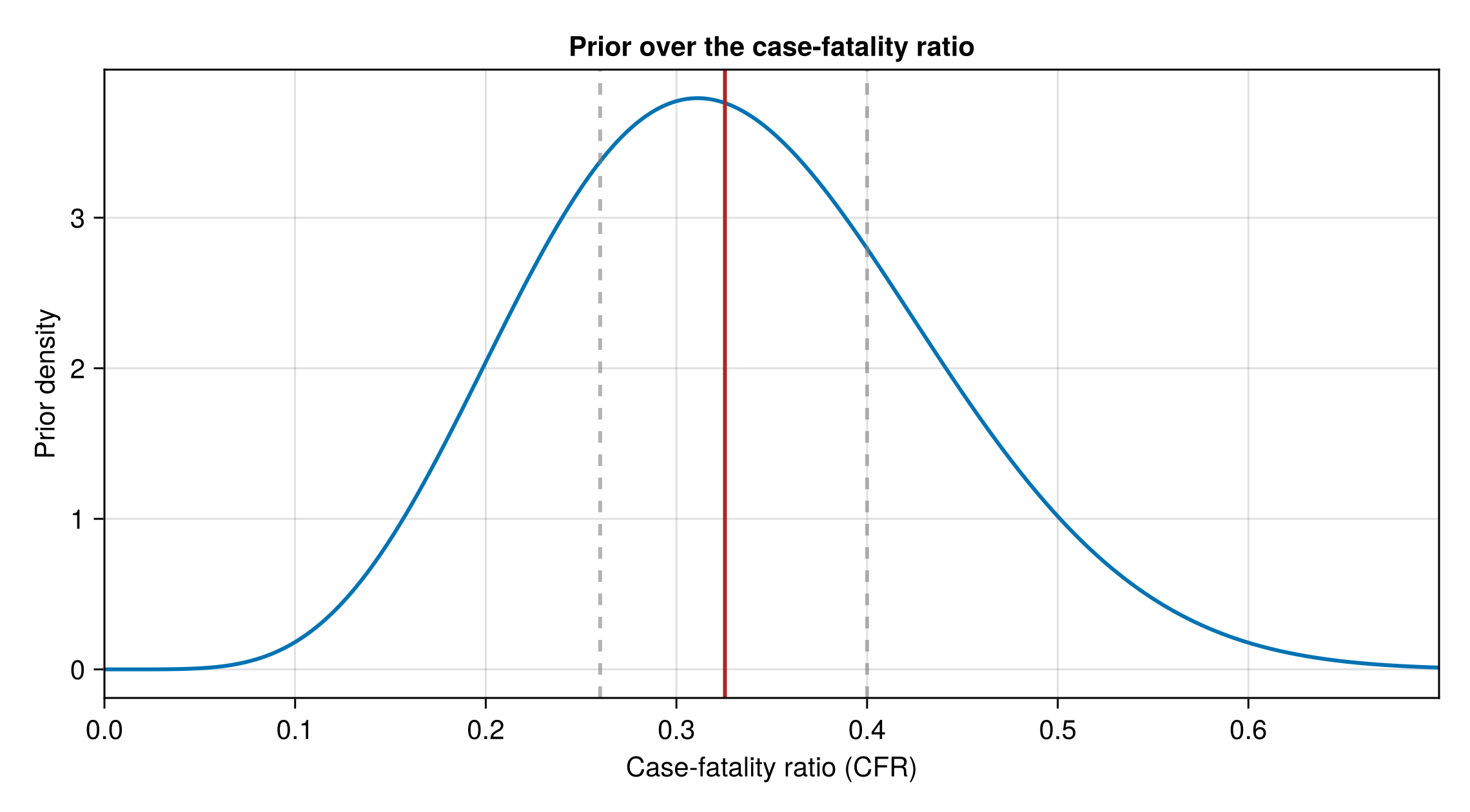
Observation models

Each observation submodel takes the shared daily onset incidence, convolves it with a sampled onset-to-event delay, and scales it by the relevant ascertainment, case-fatality ratio or positivity factor. It then reads the modelled count off the daily series at each vintage day. Likelihoods score the between-vintage increments.

Shared observation submodels

Several parameters are assumed shared across the streams: the surveillance dispersion, the ascertainment fractions, the laboratory testing priors and the traveller volume. We assume the passive-surveillance count datasets are overdispersed and share a common dispersion.

Surveillance dispersion

Each passive-surveillance count stream has its own negative-binomial dispersion, partially pooled across the streams so the sparse ones borrow strength. Following Stan prior-choice recommendations (Stan Development Team, 2024), the dispersion is sampled on the scale in non-centred log form:

so    per stream, with setting the pooling (  collapses to one shared dispersion). The population value   is the headline dispersion.

Submodel: pooled_dispersion_model

@model function pooled_dispersion_model(
        n_streams::Integer;
        mean_prior = Normal(log(0.6), 0.33),
        sd_prior = truncated(Normal(0, 0.6); lower = 0),
        centred::Bool = true
    )
    μ_log ~ mean_prior
    τ ~ sd_prior
    m = max(n_streams, 1)
    if centred
        ## Draw each stream's `log(1/sqrt(k))` directly from the population.
        ## `eps` floors the SD so a `τ ≈ 0` draw stays a proper distribution.
        log_isk ~ product_distribution(
            fill(Normal(μ_log, τ + eps(typeof(τ))), m)
        )
        inv_sqrt_k = exp.(log_isk[1:n_streams])
    else
        z ~ product_distribution(fill(Normal(0, 1), m))
        inv_sqrt_k = exp.(μ_log .+ τ .* z[1:n_streams])
    end
    k = 1.0 ./ (inv_sqrt_k .^ 2 .+ eps(eltype(inv_sqrt_k)))
    k_pop = 1.0 / (exp(μ_log)^2 + eps(typeof(float(μ_log))))
    return (; k, inv_sqrt_k, k_pop, μ_log, τ)
end

Ascertainment

Two surveillance systems detect cases: DRC passive community surveillance (the reported suspected-case count) and Uganda's point-of-entry / hospital surveillance (the exported-case count). Each captures a fraction of the true cases passing through it. The two ascertainment fractions and share a logit-scale hyperprior with mean and pooling strength , centred on a reporting fraction of . This reflects the active case-finding of a declared Ebola response rather than baseline passive surveillance:

Submodel: pooled_ascertainment_model

@model function pooled_ascertainment_model(;
        mu_prior = Normal(logit(0.75), 1.0),
        tau_prior = truncated(Normal(0, 0.5); lower = 1.0e-4)
    )
    μ_logit ~ mu_prior
    τ_logit ~ tau_prior
    z_drc ~ Normal(0, 1)
    z_uganda ~ Normal(0, 1)
    logit_p_drc = μ_logit + τ_logit * z_drc
    logit_p_uganda = μ_logit + τ_logit * z_uganda
    p_drc := logistic(logit_p_drc)
    p_uganda := logistic(logit_p_uganda)
    return (; μ_logit, τ_logit, p_drc, p_uganda)
end

Laboratory priors

We model the process of confirming cases via laboratory testing. The testing fraction is the share of suspected cases routed to the laboratory. A truly BVD specimen tests positive with the assay sensitivity , and a non-BVD specimen tests positive with the false-positive rate   from the assay specificity. We assume that more severe cases, more likely to be Ebola, are preferentially tested. This is captured by an enrichment factor that raises the tested BVD share above the suspect-pool composition early on and relaxes towards it as testing broadens. The confirmed deaths mirror this laboratory pipeline rather than enriching the case composition. The death analysed volume is specimens per suspected death, which is not a share and may exceed one for the same reason the case side is not bounded by the suspect count. Those specimens confirm at the assay positivity      . This positivity is built from the same assay sensitivity and specificity as the confirmed cases, but uses the death-pool BVD share . Confirmation runs on the altona RealStar Filovirus Screen RT-PCR (Rieger et al., 2016) rather than the Zaire-specific GeneXpert Ebola assay. The GeneXpert assay does not reliably detect Bundibugyo virus (Cepheid, 2020; Pinsky et al., 2015; Semper et al., 2016). A single assay draw is sensitive to about 85%, but a suspect is confirmed or ruled out through repeat control tests rather than one draw. The effective process sensitivity is therefore higher, about 98% with two controls, so we centre the sensitivity prior there and give it a tight spread. The specificity is high but imperfect. The severity enrichment is moderate and one-sided (triage upsamples BVD, never down). The death testing-intensity scaling is a tight log-normal centred on one, since no death-testing data grounds it:

The non-BVD background rate enters the suspected-case stream and is described with it below. The suspected deaths carry a death ascertainment    and a non-BVD death background tied to the case background by a background CFR  .

Submodel: test_positivity_model

@model function test_positivity_model(;
        lambda_prior = truncated(Normal(0.0, 1.0); lower = 0),
        fraction_tested_prior = Beta(5.0, 2.0)
    )
    λ_bg ~ lambda_prior
    τ_test ~ fraction_tested_prior
    return (; λ_bg, τ_test)
end

Submodel: test_sensitivity_model

@model function test_sensitivity_model(;
        sensitivity_prior = Beta(38.0, 2.0)
    )
    s_test ~ sensitivity_prior
    return (; s_test)
end

Submodel: test_specificity_model

@model function test_specificity_model(; specificity_prior = Beta(60.0, 2.0))
    spec ~ specificity_prior
    return (; spec)
end

Submodel: severity_enrichment_model

@model function severity_enrichment_model(;
        logodds_prior = truncated(Normal(1.5, 0.75); lower = 0),
        decay_prior = truncated(Normal(0.0, 200.0); lower = 0.0)
    )
    δ0 ~ logodds_prior
    decay_scale ~ decay_prior
    return (; δ0, decay_scale)
end

Submodel: death_testing_fraction_model

@model function death_testing_fraction_model(; fraction_prior = Beta(5.0, 2.0))
    τ_death ~ fraction_prior
    return (; τ_death)
end

Submodel: death_ascertainment_model

@model function death_ascertainment_model(;
        ascertainment_prior = Normal(logit(0.9), 0.5)
    )
    logit_p_death ~ ascertainment_prior
    p_death := logistic(logit_p_death)
    return (; p_death, logit_p_death)
end

Submodel: background_cfr_model

@model function background_cfr_model(; cfr_prior = Beta(2.0, 18.0))
    cfr_bg ~ cfr_prior
    return (; cfr_bg)
end

Traveller volume

The number of people crossing from the source area to Uganda each day sets the travel rate in the exports likelihood. We treat it as an estimated quantity rather than a fixed input. McCabe et al. Table 3 records mean weekly passenger counts across seven points of entry. The Ituri-side daily total of is a sample mean across roughly - point-of-entry-weeks. We use a Normal prior centred on with SD ( CV), truncated at zero, covering point-of-entry variation and the sitrep sampling uncertainty. The source population is kept fixed (census):

Submodel: traveller_volume_model

@model function traveller_volume_model(;
        mean::Real = ITURI_DAILY_TRAVEL,
        sd::Real = ITURI_DAILY_TRAVEL_SD
    )
    daily_travellers ~ truncated(Normal(mean, sd); lower = 0)
    return (; daily_travellers)
end

Reported cases

Reported suspected cases are the sum of two parts. The first is a BVD-driven component: the daily onsets convolved with the onset-to-report delay and scaled by the DRC ascertainment . The convolution of a daily series with a delay PMF is the lagged sum

used for every delay below. We write the BVD onset-to-report series at unit ascertainment as

The second part is an additive non-BVD background, so a suspected case need not be a true BVD infection. It is a per-day rate that follows a lognormal random walk on weekly knots around a baseline , linearly interpolated to the daily grid,

This rate is gated to zero before the surveillance onset, a report-to-receipt lead before the first suspected-case report, since the background does not exist before surveillance began. It is shared, with one tight innovation SD , between the suspected-case and suspected-death streams. Weekly knots match the reproduction-number walk and keep the background a gentle drift over a small number of innovations. The baseline carries a half-normal prior on the natural scale. A log-scale level would have a heavy right tail the background/outbreak-size degeneracy could exploit, whereas the natural-scale half-normal bounds it. It is wide enough that the laboratory positivity (only   of analysed specimens are positive) identifies the background. The background is inferred to be the majority of the suspect pool. The daily expected suspected case count is

The per-vintage increments are scored with a NegBinomial sharing the dispersion :

From SitRep 013 (27 May) INSP reclassifies suspects, so the national cumulative suspected total falls. We freeze it at 26 May and instead fit the daily new-suspect count that the confirmed-based reports publish (the "nouveaux cas suspects du jour" on report day , 4-7 June). This is a genuine daily incidence, not a cumulative total. It is scored against the modelled daily suspected count on that day directly (a single-day mean, not a between-vintage sum), with a NegBinomial sharing :

The daily report days fall strictly after the frozen cumulative series ends, so the two suspected likelihoods cover disjoint days and do not double-count. The suspected-death stream is fitted the same way. The cumulative suspected-death total freezes at 26 May, and the daily new suspected-death count ("cas suspects du jour N (M deces)", from 7 June) is scored against the modelled daily suspected-death count on each report day with a NegBinomial sharing .

Submodel: reported_cases_model

@model function reported_cases_model(
        reported_history,
        reported_cases::Union{Missing, Integer},
        onsets::AbstractVector, k::Real, p_drc::Real;
        suspected_daily_history = (; days = Int[], counts = Int[]),
        positivity = test_positivity_model(),
        background_re = nothing,
        ## Onset to a suspected case being detected/reported, from the
        ## line-list onset→admission delay (d_oa, ~4 d): a case enters
        ## surveillance when first formally seen, so one delay serves both the
        ## suspect-case and export streams. The line-list onset→notification
        ## delay (~20 d) is not used: it is assumed to reflect a longer
        ## pathway (likely confirmation and administrative processing),
        ## though what it captures is uncertain.
        onset_to_report = gamma_delay_model(
            cdf_nmax(Gamma(1.178, 3.694));
            alpha_prior = LogNormal(log(1.178), 0.25),
            theta_prior = truncated(Normal(3.694, 1.198); lower = 0.1)
        ),
        cutoff::Union{Nothing, Integer} = nothing,
        simulated = nothing
    )
    pos_state ~ to_submodel(positivity)
    report_state ~ to_submodel(onset_to_report)
    λ_bg = pos_state.λ_bg
    τ_test = pos_state.τ_test
    report_pmf = report_state.pmf

    ## Unit-ascertainment BVD onset-to-report daily series, reused by the
    ## confirmed stream.
    bvd_reports_daily = convolve_delay(onsets, report_pmf)

    n = length(bvd_reports_daily)
    nc = something(cutoff, n)
    vobs = vintage_obs(reported_history, reported_cases, nc)

    ## Daily non-BVD background. `nothing` (the renewal default) holds it at
    ## the constant scalar `λ_bg` over the grid. An injected `background_re`
    ## is the smooth daily random walk ([`background_walk_model`](@ref)),
    ## whose level `λ_mu` then overrides `λ_bg` from `positivity`.
    if background_re === nothing
        λ_bg_base = λ_bg
        bg_sigma = zero(λ_bg)
        bg_daily = fill(λ_bg, n)
    else
        bg_state ~ to_submodel(
            cutoff === nothing ? background_re(n) : background_re(n; cutoff)
        )
        λ_bg_base = bg_state.λ_mu
        bg_sigma = bg_state.σ_bg
        bg_daily = bg_state.λ
    end

    reports_daily = p_drc .* bvd_reports_daily .+ bg_daily

    modelled_increments = bin_increments(reports_daily, vobs.days)
    reported_increments ~ to_submodel(
        vintage_increments_model(
            modelled_increments,
            _sim_obs(simulated, :reported_increments, vobs.obs_increments), k
        )
    )

    ## The mean for day `d` is the single-day `reports_daily[d]`, not a
    ## between-vintage increment: this is a genuine daily incidence, so it
    ## never differences a falling cumulative.
    sd_days = suspected_daily_history.days
    sd_modelled = [reports_daily[clamp(Int(d), 1, n)] for d in sd_days]
    sd_obs = isempty(suspected_daily_history.counts) ? missing :
        collect(Int.(suspected_daily_history.counts))
    suspected_daily ~ to_submodel(
        vintage_increments_model(
            sd_modelled, _sim_obs(simulated, :suspected_daily, sd_obs), k
        )
    )

    raw_total = sum(upto(reports_daily, nc))
    expected_reports := safe_rate(raw_total)

    ## Implied per-suspected positivity at the cut-off: the BVD share of the
    ## expected suspected total.
    bvd_total = p_drc * sum(upto(bvd_reports_daily, nc))
    positivity := safe_rate(bvd_total) / expected_reports

    bg_total = sum(upto(bg_daily, nc))

    return (;
        p_drc, λ_bg = λ_bg_base, τ_test, report_pmf,
        report_mean = report_state.mean, report_sd = report_state.sd,
        bvd_reports_daily,
        reports_daily, expected_reports, positivity, bg_daily, bg_sigma,
        bg_total,
    )
end

Treatment-centre flow

The treatment-centre stream models the daily patient flow through the isolation/treatment centres: the occupied-bed count ("Patients en isolement"), the daily admissions, and the daily discharges split by outcome (in-care deaths, rule-outs and absconded). These are read from the situation-report Tableau 6 patient-movement table. Two parallel processes act on each patient. A clinical course governs how long a patient occupies a bed and how they leave it, and so sets the total occupancy and every discharge flow. A laboratory label runs alongside it and only relabels a patient from suspected to confirmed. This carves the suspect/confirmed split of the census. Death is clinical and happens under either label, so a true case may die before its test confirms it. Separating the two keeps the operational churn in the suspected pool out of the part of the occupancy the infection estimate leans on.

A proportion of the reported suspects need a bed. These admissions split into a BVD true-case inflow, admitted at a severity-skewed rate     above the base rate, and a non-BVD background inflow at the base rate,

each carried through a short suspected-to-admission delay that captures triage, transport and the wait for a bed. A patient then leaves by one of four routes. A BVD true case dies at the in-care case-fatality ratio over the admission-to-death stay, or recovers over the longer admission-to-recovery stay. A non-case is ruled out by a negative test over the rule-out stay, or absconds. The death-stay prior is the admission-to-death delay from the line-list reanalysis (Funk and Abbott, 2026), and the non-BVD rule-out stay takes the report-to-receipt laboratory turnaround.

Occupancy is the running balance of these latent events rather than a length-of-stay convolution: each day the bed stock is yesterday's stock plus the day's admissions less the day's deaths, recoveries, rule-outs and absconds. The abscond outflow drains the suspected pool at a small daily fraction of the previous day's suspected occupancy,

so the total bed demand is the forward balance

with   . The stay lives entirely in the discharge flows, each an admission stream convolved with its outcome density.

Absconding competes with the clinical exits rather than adding to them. The length-of-stay densities integrate to one, so the clinical schedules alone already account for every admitted patient, and an unthinned schedule plus an abscond outflow discharges more than was admitted. Each discharge flow is therefore thinned by the abscond survival over the stay, written here for deaths,

and likewise for recoveries and rule-outs. The discount runs on stay-day rather than calendar day: a patient resident ten days faces ten days of abscond hazard, not one for every day of the grid. Only the suspected pool absconds, so    is the probability a cohort admitted on day is still unconfirmed at stay-day , with the in-care confirmation hazard, and the discount stops once a cohort is confirmed. Background admissions are never confirmed, so   there and the rule-out schedule thins by  . Anything in the occupancy that is not infection, such as an overnight reclassification of who is counted, is modelled rather than left to bend the transmission estimate.

In-care deaths combine the two labels. A true case who dies before its test returns is a suspected death, and one who dies after is a confirmed death. The report records the two together. The death flow is therefore the in-care fatality applied to the BVD inflow over the admission-to-death stay, scored against the combined deaths directly and never gated by confirmation. The in-care fatality is a sampled log-odds modifier on the infection case-fatality ratio:

It is a fatality conditional on admission rather than a causal treatment effect, sitting below the infection case-fatality ratio where care lowers mortality. It is reported with and the overall length of stay (the death/recovery mixture mean).

The laboratory label carves the census into a confirmed and a suspected sub-stock. Confirmation relabels a true case already in a bed at the daily hazard   . The community confirmation hazard   (the share of suspects routed to the laboratory times the day's positivity) is borrowed from the confirmed-case pipeline rather than re-estimated. The in-care confirmed stock is therefore a subset of the total confirmed by construction. The confirmed-in-care stock is tracked by admission cohort. Each true-case admission carries two clocks from the day it enters a bed, a confirmation clock and a clinical-stay clock. It counts toward the confirmed census only once it has been confirmed and while it is still in a bed,

with the cumulative confirmation probability of a cohort admitted on day ,

a cumulative product along the cohort's age rather than a fixed distribution because the hazard is time-varying, and the clinical-stay survival,

the probability an admitted case is still in a bed after days, the discharge-complement of the death/recovery mixture built from the same admission-to-death and admission-to-recovery stays the discharge flows use.

Cohort tracking is needed because deaths and recoveries are observed combined across the two labels, so the data do not say which departing patients had already been confirmed. Carrying the confirmation and stay clocks separately excludes cases that die before their test returns from the confirmed pool. The suspected sub-stock is the remainder   , holding the not-yet-confirmed BVD occupancy together with the non-case occupancy awaiting rule-out. The abscond outflow drains this suspected stock at the daily fraction . Recoveries among the confirmed (the published recovery total) are the confirmed subset of recoveries and are modelled as a separate confirmed-recovery stream (below).

Capacity enters only as a censored observation. The latent demand is never capped, because the demand is the quantity of interest. The bed capacity is a non-decreasing random walk on weekly knots, since beds are added over the response and not taken away. It is pinned by the implied bed count, the reported occupancy divided by the reported occupancy rate (about rising to beds over 9-13 June). The occupied beds are scored as the latent demand right-censored at the recorded implied capacity, so demand above a saturated capacity is left uncensored. The censoring bound is fixed recorded data, so it does not drift with the modelled capacity. The occupancy and a flow stream are scored as

with each flow mean the matching modelled event series (the admissions, the in-care deaths, the rule-outs and the absconds), all sharing the treatment dispersion . The implied capacity is carried by a NegBinomial of its own. Demand above a saturated capacity is only partially identified, since the occupancy reveals that demand was at least the beds filled but not how much more. The bed shortfall above capacity is therefore informed by the demand model and its priors rather than measured. Bed demand is the uncapped diagnostic, and the model exposes the cut-off occupancy on the reported scale (the demand plus the reclassification offset, floored at zero and capped at the cut-off beds), the cut-off bed demand (the need under unconstrained supply), the demand plus offset above the cut-off beds (the bed shortfall) and the utilisation. The capacity walk is an ingredient of the beds rather than the beds reported. With one patch the cut-off beds are the modelled capacity floored at the last recorded capacity. With several, each province's cut-off beds are its modelled capacity floored at its last recorded effective beds, its occupancy is its demand share of the national demand plus offset capped at those beds, and the rest is its shortfall. The national beds, occupancy and shortfall are the sums over the provinces. Patients do not move between provinces, so the national occupancy   is below   whenever a province is over its beds.

The fitted occupancy series is the all-patients column from 1 June (SitRep 018) onward. From 13 June the report adds a two-row breakdown into confirmed and suspected beds that sums to the total each day. The total-occupancy term is the backbone present from 1 June. The daily flows and the confirmed/suspected census add likelihood on the days they exist, scored per day as either the total or the split, so the total and its parts are never both counted on one day. The early window, with only the total occupancy reported, fits the backbone alone while the latent admissions still drive the stock. The split is scored only where the borrowed confirmation hazard is non-zero, that is, where the laboratory pipeline of the full model supplies it.

One reporting artefact is modelled, on identified days only: an overnight reclassification of the total. The published start-of-day in-bed count is differenced against the previous report day's occupancy, and a day whose gap exceeds a threshold is flagged as a break day. One step is fitted per flagged day, with a prior centred on that day's observed gap but free to move, so the fit can attribute part of a gap to genuine change in demand. The steps accumulate into a persistent additive offset on the modelled total occupancy, carried forward to every later day. This offset absorbs the overnight gap without bending the reproduction number to chase it. The split does not change the occupancy before 13 June, since no breakdown is published there and the total backbone carries that window.

The reports also print the patients in isolation and the beds by province, for whichever provinces report that day. Both enter as splits of the printed sum of the provinces present, so the national terms above keep their likelihoods on every day. Each patch's BVD admissions are its BVD reports through the admission delay, re-split so that together they are the national BVD admissions and each patch carries the case composition's relative ascertainment (defined with the province compositions below):

Each patch's approximate stock is these admissions through the clinical-stay survival plus its share of the non-BVD admissions through the rule-out stay, and the national demand is shared out in proportion:

is the rule-out cohort's exact survival under the running balance (36), absconding included. The confirmation relabelling and the absconding of unconfirmed cases are shared across patches, so they cancel from the shares only approximately. Each patch's capacity on day is a share of the national capacity walk. Beds are allocated in response to cases, so we centre the share on the patch's modelled cumulative admissions to date, BVD and background together:

normalised over the patches each day, with the sum-to-zero basis of the Rt deviations. A shift shared by every patch cancels in the normalisation, so the deviations sum to zero and no patch is a reference. The floor is one admission, so a patch with no admissions yet still holds some beds. The deviations are static, and the share moves over time only through its centre. On a day on which the provinces print, taken in patch order, the printed counts are allocated across them by the stick-breaking of equation (54):

with   on . The occupancy is split on the uncapped demand, since a province can print more patients than beds. The recorded province beds are the effective beds: the printed beds, or where more patients are held, the larger of the patients and the beds implied by the printed occupancy rate. Each day's 24h admissions are split the same way on each patch's modelled admissions  , with their own . The occupancy split is scored weekly and the bed split on the days a count changes, since a stock reprinted daily is not a fresh draw. The admissions are a flow, so every day is scored.

Submodel: treatment_flow_model

@model function treatment_flow_model(
        isolation_history,
        bvd_reports_daily::AbstractVector,
        bg_daily::AbstractVector,
        p_drc::Real,
        CFR::Real;
        capacity_history = (; days = Int[], counts = Int[]),
        admissions_history = (; days = Int[], counts = Int[]),
        deaths_history = (; days = Int[], counts = Int[]),
        ruleout_history = (; days = Int[], counts = Int[]),
        absconded_history = (; days = Int[], counts = Int[]),
        ## Tableau 6 occupancy split (`dont confirmés` / `dont suspects`): two
        ## census series scored in place of the total occupancy on the days
        ## they are present, only when the confirmation hazard is non-zero.
        confirmed_incare_history = (; days = Int[], counts = Int[]),
        suspect_incare_history = (; days = Int[], counts = Int[]),
        ## Daily in-care confirmation hazard `τ_test · p_pos` borrowed from
        ## the lab pipeline ([`confirmed_cases_model`](@ref)). `nothing`
        ## (standalone, no lab stream) gives a zero hazard, so the confirmed
        ## sub-stock stays empty and the suspect sub-stock carries the whole
        ## occupancy.
        conf_hazard_daily::Union{Nothing, AbstractVector} = nothing,
        ## The priors and delay submodels the keywords below default to.
        defaults = treatment_flow_defaults(),
        admission = defaults.admission,
        severity = defaults.severity,
        capacity = bed_capacity_walk_model,
        dispersion = defaults.dispersion,
        ## Occupancy / flow dispersion can be injected from the joint composer's
        ## pooled set (`k_external`). Standalone it samples its own.
        k_external::Union{Nothing, Real} = nothing,
        cfr_modifier_prior = defaults.cfr_modifier_prior,
        abscond_prior = defaults.abscond_prior,
        incare_confirm_log_prior = defaults.incare_confirm_log_prior,
        admission_delay = defaults.admission_delay,
        death_los = defaults.death_los,
        recovery_los = defaults.recovery_los,
        ruleout_los = defaults.ruleout_los,
        ## Opt-in occupancy reclassification-break days (grid indices). A level
        ## step is fitted into the modelled total at each, absorbing a
        ## measurement-basis discontinuity in the isolation series. See
        ## `cumulative_occupancy_offset`.
        occupancy_break_days::AbstractVector{<:Integer} = Int[],
        ## Prior sd of each occupancy break step (beds), centred on zero.
        occupancy_break_sd::Real = 25.0,
        ## Per-patch BVD reports `(n_patches × n)`, the rows summing to
        ## `bvd_reports_daily`. `nothing` is one patch.
        bvd_reports_matrix::Union{Nothing, AbstractMatrix} = nothing,
        ## Share of the non-BVD background in each patch, summing to one
        ## ([`background_split_model`](@ref)).
        background_split::AbstractVector{<:Real} = [1.0],
        ## Relative case ascertainment by patch (the case composition's),
        ## which splits the national BVD admissions by ascertainment-weighted
        ## incidence. Ones leaves the split on incidence alone.
        patch_ascertainment::AbstractVector{<:Real} = ones(
            length(background_split)
        ),
        ## Province occupancy, bed and 24h admission rows,
        ## `(; days, patches, counts)` from `province_care_observations`, or
        ## `nothing`. Scored as splits of the printed sum of the provinces
        ## present each day.
        province_isolation = nothing,
        province_capacity = nothing,
        province_admissions = nothing,
        patch_capacity = patch_capacity_share_model,
        province_split_rho_prior = truncated(
            Normal(0, 0.1); lower = 0, upper = 1
        ),
        cutoff::Union{Nothing, Integer} = nothing,
        simulated = nothing
    )
    adm_state ~ to_submodel(admission)
    p_iso = adm_state.p_iso
    sev_state ~ to_submodel(severity)
    ## BVD suspects are admitted at a higher rate than non-BVD rule-outs,
    ## skewed up from `p_iso` by the severity log-odds `δ_iso`.
    p_iso_bvd = logistic(logit(p_iso) + sev_state.δ_iso)
    if k_external === nothing
        disp_state ~ to_submodel(dispersion)
        k = disp_state.k
    else
        k = k_external
    end
    n = length(bvd_reports_daily)
    nc = something(cutoff, n)
    ## `β_iso` is identified by the in-care death flow (Tableau 6 décédés)
    ## relative to admissions and occupancy. The recovered-among-confirmed
    ## ("cumul guéris") stream is modelled separately off the confirmed cases
    ## ([`recovered_model`](@ref)), since guéris is the
    ## confirmed-and-discharged subset, not all in-care recoveries.
    β_iso ~ cfr_modifier_prior
    CFR_iso = logistic(logit(CFR) + β_iso)
    ## Time-varying bed capacity `C(t)` (a random walk), started at the first
    ## day with occupancy or capacity data.
    cap_obs_days = vcat(
        Int.(isolation_history.days),
        Int.(capacity_history.days)
    )
    cap_start = isempty(cap_obs_days) ? 1 : minimum(cap_obs_days)
    np = bvd_reports_matrix === nothing ? 1 : size(bvd_reports_matrix, 1)
    length(background_split) == np || error(
        "treatment_flow_model: $(length(background_split)) background " *
            "shares for $(np) patches."
    )
    ## The per-patch demand and capacity shares are built only when a
    ## province split scores them; without province rows the stream is the
    ## national one whatever the patch count.
    split_occ = np > 1 && province_isolation !== nothing &&
        !isempty(province_isolation.days)
    split_cap = np > 1 && province_capacity !== nothing &&
        !isempty(province_capacity.days)
    split_adm = np > 1 && province_admissions !== nothing &&
        !isempty(province_admissions.days)
    by_patch = split_occ || split_cap || split_adm
    cap_state ~ to_submodel(
        cutoff === nothing ? capacity(n; start = cap_start) :
            capacity(n; start = cap_start, cutoff)
    )
    C = cap_state.C
    ## Recorded beds the cut-off and forecast beds are floored at: each
    ## province's last effective beds with province rows, else the national
    ## recorded cap on the last occupancy day.
    bed_floors = by_patch ? _province_bed_floors(province_capacity, np, nc) :
        _national_bed_floor(capacity_history, isolation_history)
    adm_delay_state ~ to_submodel(admission_delay)
    death_los_state ~ to_submodel(death_los)
    recovery_los_state ~ to_submodel(recovery_los)
    ruleout_los_state ~ to_submodel(ruleout_los)
    ## Abscond (loss-to-follow-up) drains the suspect pool at a small daily
    ## fraction κ of the previous-day suspect occupancy.
    abscond_frac ~ abscond_prior
    κ = abscond_frac

    ## Opt-in reclassification-break offset Δ(t), absorbing the `au-lit-J-1`
    ## versus `Fin-J` discontinuity in the observed isolation series. Each
    ## step is sampled non-centred around zero, so the fit partitions it into
    ## reporting artefact and real demand. Only break days on or before an
    ## observed occupancy day can move the likelihood, so later ones are
    ## dropped rather than sampling an inert step.
    iso_last = isempty(isolation_history.days) ? 0 :
        maximum(Int.(isolation_history.days))
    brk_days = [Int(d) for d in occupancy_break_days if Int(d) <= iso_last]
    if isempty(brk_days)
        b = Float64[]
    else
        occupancy_step ~ product_distribution(
            fill(Normal(0, 1), length(brk_days))
        )
        b = occupancy_break_sd .* occupancy_step
    end
    break_grid_days = brk_days
    occ_break_offset = cumulative_occupancy_offset(1:n, break_grid_days, b)

    ## Admission inflow through the suspected→admission delay, split into BVD
    ## true-case (`p_iso_bvd`) and non-BVD (`p_iso`) inflows. Uncapped latent
    ## demand. Capacity enters only as a censoring bound below.
    A_bvd = convolve_delay(
        p_iso_bvd .* p_drc .* bvd_reports_daily,
        adm_delay_state.pmf
    )
    A_bg = convolve_delay(p_iso .* bg_daily, adm_delay_state.pmf)
    if eltype(A_bvd) === Any
        A_bvd = convert(Vector{eltype(C)}, A_bvd)
        A_bg = convert(Vector{eltype(C)}, A_bg)
    end

    admit_daily = A_bvd .+ A_bg

    ## Community confirmation hazard `τ_test · p_pos` borrowed from the lab
    ## pipeline. `nothing` (standalone) gives a zero hazard.
    borrowed_hazard = if conf_hazard_daily === nothing
        zeros(eltype(A_bvd), n)
    elseif eltype(conf_hazard_daily) === Any
        convert(Vector{eltype(C)}, conf_hazard_daily)
    else
        conf_hazard_daily
    end

    ## The split census is identified only when the borrowed hazard is
    ## non-zero (a lab stream supplies it). With a structural zero the
    ## confirmed sub-stock is empty, so the split likelihood no-ops and
    ## those days stay on the total.
    split_active = any(
        >(zero(eltype(borrowed_hazard))), upto(borrowed_hazard, nc)
    )

    ## In-care confirmation-rate modifier ρ = exp(γ_conf) on the borrowed
    ## hazard. Sampled only when the hazard is non-zero, so no unidentified
    ## dimension is added when the split is absent.
    if split_active
        incare_confirm_log ~ incare_confirm_log_prior
    else
        incare_confirm_log = zero(eltype(borrowed_hazard))
    end
    ρ_conf = exp(incare_confirm_log)
    conf_hazard = ρ_conf .* borrowed_hazard

    ## Label-independent clinical discharge events. Deaths and recoveries
    ## split `A_bvd` by `CFR_iso`, and rule-outs discharge `A_bg`. Each
    ## schedule is thinned by the abscond survival so absconding competes with
    ## the clinical exits instead of adding to them. True cases stop being at
    ## risk once confirmed, so theirs carry the confirmation hazard
    ## ([`abscond_thinned_flow`](@ref)). Background admissions are never
    ## confirmed, so a flat cohort-age thinning is exact for the rule-outs
    ## ([`abscond_thinned`](@ref)).
    deaths_daily, recover_daily = abscond_thinned_flows(
        CFR_iso .* A_bvd, death_los_state.pmf,
        (one(CFR_iso) - CFR_iso) .* A_bvd, recovery_los_state.pmf,
        κ, conf_hazard
    )
    ruleout_daily = convolve_delay(
        A_bg,
        abscond_thinned(ruleout_los_state.pmf, κ)
    )
    ## Still-in-a-bed survival for the two-clock confirmed sub-stock below.
    ## `two_clock_confirmed` takes one schedule for every cohort, so it cannot
    ## carry the admission-day-dependent abscond survival the flows above use.
    ## The flat cohort-age thinning over-discounts by the confirmed share,
    ## second order against the confirmation hazard the sub-stock is built
    ## from.
    dpmf = abscond_thinned(death_los_state.pmf, κ)
    rpmf = abscond_thinned(recovery_los_state.pmf, κ)

    ## Forward running-balance occupancy: total demand and the BVD/non-case
    ## stocks. The scored abscond flow is recomputed below off the two-clock
    ## suspect stock.
    acc = accumulate_occupancy(
        A_bvd, A_bg, deaths_daily, recover_daily,
        ruleout_daily, κ, conf_hazard
    )
    demand_raw = acc.demand
    O_bvd = acc.O_bvd

    ## Two-clock confirmed-in-care sub-stock: cohort-tracked
    ## confirmed-and-present prevalence, exact in the fast-death tail where
    ## the running balance's proportional drain is only mean-field. Demand
    ## and `O_bvd` stay as `accumulate_occupancy` built them, while `O_conf`
    ## (and `O_susp = D − O_conf`) is replaced.
    S_clin = clinical_stay_survival(dpmf, rpmf, CFR_iso)
    O_conf_raw = two_clock_confirmed(A_bvd, conf_hazard, S_clin)
    demand = _typed_as(demand_raw, C)

    ## Per-patch admissions, bed demand and capacity for the province
    ## splits and the province forecast. The
    ## demand is the national demand shared out by each patch's stock of
    ## admissions through the stays. The capacity is the national walk times
    ## a daily share centred on each patch's cumulative admissions
    ## ([`patch_capacity_share_model`](@ref)). The stock falls as patients
    ## leave; the cumulative admissions never fall. With one patch both are
    ## the national series as one row.
    if by_patch
        A_bvd_patch = _patch_bvd_admissions(
            bvd_reports_matrix, patch_ascertainment, p_iso_bvd, p_drc,
            adm_delay_state.pmf
        )
        demand_patch = _patch_demand(
            A_bvd_patch, A_bg, background_split, S_clin,
            ruleout_los_state.pmf, κ, demand
        )
        admit_patch = _patch_admissions(A_bvd_patch, A_bg, background_split)
        cap_share_state ~ to_submodel(patch_capacity(admit_patch))
        cap_shares = cap_share_state.s
        cap_pooling_sd = cap_share_state.pooling_sd
    else
        demand_patch = reshape(demand, 1, :)
        admit_patch = reshape(admit_daily, 1, :)
        cap_shares = ones(eltype(C), 1, n)
        cap_pooling_sd = zero(eltype(C))
    end
    C_patch = cap_shares .* reshape(C, 1, :)

    ## Reclassification offset Δ(t), added to the modelled census total only.
    ## Demand (the diagnostic) stays the un-offset latent stock.
    occ_offset = _typed_as(occ_break_offset, C)
    ## `O_conf ≤ O_bvd` holds by construction; the census clamps it to guard
    ## any prior draw. Absconds drain the two-clock suspect stock, and the
    ## confirmed and suspect census means sum to the offset total.
    census = incare_census(
        demand, _typed_as(O_bvd, C), _typed_as(O_conf_raw, C), κ,
        occ_offset
    )
    abscond_daily = census.abscond
    occ_obs_total = census.total
    conf_split = census.confirmed
    susp_split = census.suspect

    ## Occupancy likelihood: NegativeBinomial around the latent demand,
    ## right-censored at the implied-capacity bound. Days with a published
    ## split are scored as the two sub-stocks below instead, so the total and
    ## its parts are never both scored on one day.
    split_days = split_active ? Set(Int.(confirmed_incare_history.days)) :
        Set{Int}()
    iso_all_days = isolation_history.days
    iso_keep = [!(Int(d) in split_days) for d in iso_all_days]
    iso_days = iso_all_days[iso_keep]
    iso_obs = isempty(isolation_history.counts) ? missing :
        collect(Int.(isolation_history.counts))[iso_keep]
    iso_means = [occ_obs_total[clamp(Int(d), 1, n)] for d in iso_days]
    iso_ceil = censoring_cap(iso_days, iso_obs, capacity_history)
    isolation ~ to_submodel(
        censored_occupancy_model(
            iso_means, iso_ceil, _sim_obs(simulated, :isolation, iso_obs), k
        )
    )

    ## Capacity likelihood: the implied bed count is a noisy observation of
    ## C(t).
    cap_days = capacity_history.days
    cap_modelled = [C[clamp(Int(d), 1, n)] for d in cap_days]
    cap_obs = isempty(capacity_history.counts) ? missing :
        collect(Int.(capacity_history.counts))
    bed_capacity ~ to_submodel(
        vintage_increments_model(
            cap_modelled, _sim_obs(simulated, :bed_capacity, cap_obs), k
        )
    )

    ## Province splits of the occupancy and of the beds, conditional on the
    ## printed sum of the provinces present each day. The national tile and
    ## the national implied capacity above keep their likelihoods, so these
    ## add only the spatial split. Occupancy is split on the uncapped
    ## per-patch demand: the printed bed counts do not cover every structure
    ## patients are held in, so a province can print more patients than
    ## beds (Nord-Kivu from SitRep 124, 376 in-patients against 228 normed
    ## beds), and a cap at the walk would read that as a smaller share.
    ## Saturation is reported through the per-patch utilisation and
    ## shortfall instead.
    occupancy_split_rho = 0.0
    if split_occ
        occupancy_split_rho ~ province_split_rho_prior
        occupancy_split ~ to_submodel(
            province_split_model(
                merge(
                    province_isolation,
                    (;
                        counts = _sim_obs(
                            simulated, :occupancy_split,
                            province_isolation.counts
                        ),
                    )
                ),
                demand_patch, occupancy_split_rho
            )
        )
    end
    capacity_split_rho = 0.0
    if split_cap
        capacity_split_rho ~ province_split_rho_prior
        capacity_split ~ to_submodel(
            province_split_model(
                merge(
                    province_capacity,
                    (;
                        counts = _sim_obs(
                            simulated, :capacity_split,
                            province_capacity.counts
                        ),
                    )
                ),
                C_patch, capacity_split_rho
            )
        )
    end
    ## Admissions are a flow, so every day is scored.
    admissions_split_rho = 0.0
    if split_adm
        admissions_split_rho ~ province_split_rho_prior
        admissions_split ~ to_submodel(
            province_split_model(
                merge(
                    province_admissions,
                    (;
                        counts = _sim_obs(
                            simulated, :admissions_split,
                            province_admissions.counts
                        ),
                    )
                ),
                admit_patch, admissions_split_rho
            )
        )
    end

    ## Split likelihoods, guarded by `split_active` so they no-op when the
    ## hazard is structurally zero.
    ci_days = split_active ? confirmed_incare_history.days : Int[]
    ci_obs = (!split_active || isempty(confirmed_incare_history.counts)) ?
        missing : collect(Int.(confirmed_incare_history.counts))
    confirmed_incare_obs ~ to_submodel(
        vintage_increments_model(
            [conf_split[clamp(Int(d), 1, n)] for d in ci_days],
            _sim_obs(simulated, :confirmed_incare_obs, ci_obs), k
        )
    )
    si_days = split_active ? suspect_incare_history.days : Int[]
    si_obs = (!split_active || isempty(suspect_incare_history.counts)) ?
        missing : collect(Int.(suspect_incare_history.counts))
    suspect_incare_obs ~ to_submodel(
        vintage_increments_model(
            [
                max(susp_split[clamp(Int(d), 1, n)], zero(eltype(susp_split)))
                    for d in si_days
            ], _sim_obs(simulated, :suspect_incare_obs, si_obs), k
        )
    )
    ## Optional daily Tableau 6 flow likelihoods, each a no-op on empty history.
    dth_days = deaths_history.days
    dth_obs = isempty(deaths_history.counts) ? missing :
        collect(Int.(deaths_history.counts))
    incare_deaths ~ to_submodel(
        vintage_increments_model(
            [deaths_daily[clamp(Int(d), 1, n)] for d in dth_days],
            _sim_obs(simulated, :incare_deaths, dth_obs), k
        )
    )
    ro_days = ruleout_history.days
    ro_obs = isempty(ruleout_history.counts) ? missing :
        collect(Int.(ruleout_history.counts))
    ruleouts ~ to_submodel(
        vintage_increments_model(
            [ruleout_daily[clamp(Int(d), 1, n)] for d in ro_days],
            _sim_obs(simulated, :ruleouts, ro_obs), k
        )
    )
    adm_h_days = admissions_history.days
    adm_h_obs = isempty(admissions_history.counts) ? missing :
        collect(Int.(admissions_history.counts))
    admissions ~ to_submodel(
        vintage_increments_model(
            [admit_daily[clamp(Int(d), 1, n)] for d in adm_h_days],
            _sim_obs(simulated, :admissions, adm_h_obs), k
        )
    )
    ab_days = absconded_history.days
    ab_obs = isempty(absconded_history.counts) ? missing :
        collect(Int.(absconded_history.counts))
    absconded ~ to_submodel(
        vintage_increments_model(
            [abscond_daily[clamp(Int(d), 1, n)] for d in ab_days],
            _sim_obs(simulated, :absconded, ab_obs), k
        )
    )

    ## Cut-off reported quantities, by patch and summed to national. Each
    ## patch's beds are its modelled capacity floored at its recorded beds.
    ## Its occupancy is its demand share of the mean the reported occupancy
    ## is scored around (the demand plus the reclassification offset,
    ## floored at zero), capped at its beds; the rest is its shortfall.
    ## Patients do not move between patches, so the national occupancy is
    ## the sum of the capped patches. Bed demand is the latent stock.
    z0 = zero(eltype(C))
    dem_T = isempty(demand) ? z0 : demand[nc]
    cut = cutoff_occupancy(
        isempty(occ_obs_total) ? z0 : occ_obs_total[nc],
        demand_patch[:, nc], C_patch[:, nc], bed_floors
    )
    beds_T = sum(cut.beds)
    occ_T = sum(cut.occupancy)
    overall_los = CFR_iso * death_los_state.mean +
        (one(CFR_iso) - CFR_iso) * recovery_los_state.mean
    ## Each cut-off quantity below is both `:=`-tracked onto the chain and
    ## returned, so it is bound once and used twice. Computing it twice puts
    ## the work on the gradient path twice, and lets an edit to one copy
    ## leave the chain and the returned value disagreeing.
    isolation_T = safe_rate(occ_T)
    bed_demand_T = safe_rate(dem_T)
    expected_isolation := isolation_T
    expected_bed_demand := bed_demand_T
    ## Cut-off daily flows: each modelled daily series on the cut-off day,
    ## for admissions, in-care deaths and rule-outs.
    admissions_T = safe_rate(isempty(admit_daily) ? z0 : admit_daily[nc])
    incare_deaths_T = safe_rate(
        isempty(deaths_daily) ? z0 :
            deaths_daily[nc]
    )
    ruleouts_T = safe_rate(isempty(ruleout_daily) ? z0 : ruleout_daily[nc])
    expected_admissions := admissions_T
    expected_incare_deaths := incare_deaths_T
    expected_ruleouts := ruleouts_T
    shortfall_T = safe_rate(sum(cut.shortfall))
    bed_shortfall := shortfall_T
    bed_utilisation := isolation_T / safe_rate(beds_T)
    isolation_severity := sev_state.δ_iso
    isolation_bvd_admission := p_iso_bvd
    incare_cfr := CFR_iso
    incare_cfr_modifier := β_iso
    treatment_overall_los := overall_los
    conf_incare_T = isempty(conf_split) ? z0 : conf_split[nc]
    susp_incare_T = isempty(susp_split) ? z0 : max(susp_split[nc], z0)
    conf_incare_rate = safe_rate(conf_incare_T)
    susp_incare_rate = safe_rate(susp_incare_T)
    expected_confirmed_incare := conf_incare_rate
    expected_suspect_incare := susp_incare_rate
    incare_confirmed_share := conf_incare_rate / bed_demand_T
    ## Raw, since ρ can exceed one. ρ < 1 means occupied suspects are
    ## confirmed slower than the borrowed community hazard, held for repeated
    ## exclusion testing.
    incare_confirm_modifier := ρ_conf
    ## How much of the observed reclassification the model absorbed as a
    ## reporting artefact, the rest carried by real demand. Fitted and
    ## possibly negative, so reported raw rather than through `safe_rate`.
    break_T = isempty(occ_break_offset) ? z0 : occ_break_offset[nc]
    occupancy_break := break_T

    return (;
        p_iso, p_iso_bvd, δ_iso = sev_state.δ_iso,
        CFR_iso, β_iso, capacity = beds_T,
        beds_patch_T = cut.beds, occupancy_patch_T = cut.occupancy,
        shortfall_patch_T = cut.shortfall,
        death_los_mean = death_los_state.mean,
        recovery_los_mean = recovery_los_state.mean,
        ruleout_los_mean = ruleout_los_state.mean,
        admission_delay_mean = adm_delay_state.mean,
        overall_los, abscond_frac, k_isolation = k,
        demand, isolation, C,
        occupancy_mean = occ_obs_total,
        demand_patch, admit_patch, capacity_patch = C_patch,
        capacity_series = C,
        capacity_shares = cap_shares, capacity_pooling_sd = cap_pooling_sd,
        occupancy_split_rho, capacity_split_rho, admissions_split_rho,
        deaths_daily, recover_daily, ruleout_daily, admit_daily,
        abscond_daily,
        break_steps = b, break_offset = occ_break_offset,
        break_grid_days,
        occupancy_break = break_T,
        confirmed_incare = conf_split, suspect_incare = susp_split,
        incare_confirm_modifier = ρ_conf,
        expected_confirmed_incare = conf_incare_rate,
        expected_suspect_incare = susp_incare_rate,
        expected_isolation = isolation_T,
        expected_bed_demand = bed_demand_T,
        bed_shortfall = shortfall_T,
        expected_admissions = admissions_T,
        expected_incare_deaths = incare_deaths_T,
        expected_ruleouts = ruleouts_T,
    )
end

Submodel: patch_capacity_share_model

@model function patch_capacity_share_model(
        admissions::AbstractMatrix{<:Real};
        admission_floor::Real = 1.0,
        pooling_sd_prior = truncated(Normal(0, 1); lower = 0),
        offset_prior = Normal(0, 1),
        basis = sum_to_zero_basis(max(size(admissions, 1), 1))
    )
    np, n = size(admissions)
    if np <= 1
        return (; s = ones(Float64, max(np, 1), n), pooling_sd = 0.0)
    end
    admission_floor > 0 || error(
        "patch_capacity_share_model: admission_floor must be positive, " *
            "got $(admission_floor)."
    )
    τ_cap ~ pooling_sd_prior
    z_cap ~ product_distribution(fill(offset_prior, np - 1))
    dev = sum_to_zero(sum_to_zero_factor(basis, τ_cap), z_cap)
    s = _admission_centred_shares(admissions, dev, admission_floor)
    return (; s, pooling_sd = τ_cap)
end

Suspected deaths

Suspected deaths are the ascertained, CFR-weighted convolution of the daily onsets with the onset-to-death PMF , plus a non-BVD background. This is modelled on the incidence scale. The death history ends at the cut-off, so the cut-off total is the final increment and is not scored separately. A fatal BVD infection enters the suspected-death count only when ascertained. The BVD deaths therefore carry a death ascertainment , the death analogue of the case ascertainment , with an informative prior centred high (a death is more reliably reported than a living suspect). The non-BVD background suspected deaths are a background CFR applied to the per-day non-BVD suspected-case background , lagged by the same onset-to-death delay so a background death follows its background case. The daily death series is

The per-vintage increments are scored with a NegBinomial sharing the dispersion :

Submodel: deaths_model

@model function deaths_model(
        deaths_history,
        total_deaths::Union{Missing, Integer},
        onsets::AbstractVector, k::Real;
        suspected_daily_deaths_history = (; days = Int[], counts = Int[]),
        cfr = cfr_model(),
        ascertainment = death_ascertainment_model(),
        case_bg_daily = nothing,
        background_cfr = background_cfr_model(),
        ## nmax covers 98% of the convolved onset->death sum (the two atomic
        ## Gammas moment-matched to a single Gamma only for the truncation).
        onset_to_death = onset_to_death_model(
            cdf_nmax(Gamma(3.33, 3.83));
            oa_alpha_prior = LogNormal(log(1.178), 0.25),
            oa_theta_prior = truncated(Normal(3.694, 1.198); lower = 0.1),
            ad_alpha_prior = truncated(Normal(2.151, 0.604); lower = 0.01),
            ad_theta_prior = truncated(Normal(3.906, 1.381); lower = 0.1)
        ),
        cutoff::Union{Nothing, Integer} = nothing,
        simulated = nothing
    )
    cfr_state ~ to_submodel(cfr)
    od_state ~ to_submodel(onset_to_death)
    asc_state ~ to_submodel(ascertainment)
    CFR = cfr_state.CFR
    p_death = asc_state.p_death
    bvd_deaths_daily = convolve_delay(onsets, (p_death * CFR) .* od_state.pmf)

    n = length(bvd_deaths_daily)
    nc = something(cutoff, n)
    vobs = vintage_obs(deaths_history, total_deaths, nc)

    ## `λ_bg_death` is the mean daily background death rate.
    if case_bg_daily !== nothing
        bgcfr_state ~ to_submodel(background_cfr)
        cfr_bg = bgcfr_state.cfr_bg
        bg_death_daily = convolve_delay(case_bg_daily, cfr_bg .* od_state.pmf)
        λ_bg_death = sum(upto(bg_death_daily, nc)) / nc
        bg_death_sigma = zero(CFR)
    else
        cfr_bg = zero(CFR)
        λ_bg_death = zero(CFR)
        bg_death_sigma = zero(CFR)
        bg_death_daily = fill(zero(CFR), n)
    end

    deaths_daily = bvd_deaths_daily .+ bg_death_daily

    modelled_increments = bin_increments(deaths_daily, vobs.days)
    death_increments ~ to_submodel(
        vintage_increments_model(
            modelled_increments,
            _sim_obs(simulated, :death_increments, vobs.obs_increments), k
        )
    )

    ## The mean for day `d` is the single-day `deaths_daily[d]`, not a
    ## between-vintage increment: this is a genuine daily count, so it never
    ## differences a falling cumulative.
    sdd_days = suspected_daily_deaths_history.days
    sdd_modelled = [deaths_daily[clamp(Int(d), 1, n)] for d in sdd_days]
    sdd_obs = isempty(suspected_daily_deaths_history.counts) ? missing :
        collect(Int.(suspected_daily_deaths_history.counts))
    suspected_daily_deaths ~ to_submodel(
        vintage_increments_model(
            sdd_modelled,
            _sim_obs(simulated, :suspected_daily_deaths, sdd_obs), k
        )
    )

    raw_total = sum(upto(deaths_daily, nc))
    expected_deaths_T := safe_rate(raw_total)
    bg_death_total = sum(upto(bg_death_daily, nc))

    return (;
        CFR, p_death, cfr_bg, od_pmf = od_state.pmf, deaths_daily,
        bvd_deaths_daily, expected_deaths_T, λ_bg_death, bg_death_sigma,
        bg_death_daily, bg_death_total,
    )
end

Laboratory pipeline

The laboratory pipeline fits a single analysed-specimen volume. It is the suspected daily pipeline (  plus the non-BVD background ) carried through the report-to-analysed delay , thinned by the testing fraction (the share of suspected cases routed to the laboratory), and multiplied by the specimens analysed per suspect sampled ,

exceeds one because repeat exclusion testing, swabbed community deaths and screened contacts all put specimens into the laboratory denominator without adding a reported suspect.

This analysed volume is gated to zero before the testing onset. The first confirmed vintage is treated as the baseline and the early confirmed increments are scored from it. The suspected-case count itself is not gated, as those cases did accumulate over the cryptic phase.

The death volume scales the modelled case analysed volume at the per-day suspected death-to-case ratio (described in the confirmed deaths section below). The two therefore share the laboratory capacity onset.

The per-vintage increments are scored against the cumulative analysed series with a NegBinomial sharing the dispersion :

The confirmed positives in each laboratory window are scored as a Binomial of the observed specimens-analysed denominator with a per-window tested-positive probability . Where no analysed count is observed (the early and unanchored windows), the modelled volume is the denominator instead. We tie that probability to the composition of the tested pool, so the confirmed data help identify the non-BVD background. The suspect-pool composition is the BVD share among the specimens analysed in the window, carried through the same delay as the volume so composition and volume share one clock:

The tested BVD share raises by the decaying severity enrichment :

The false-positive term therefore carries the non-BVD share, and the laboratory data identify the background:

with the cumulative modelled laboratory volume at window , the clock on which the enrichment decays. The confirmed vintages before the first and after the last laboratory date carry no observed analysed denominator. They are scored as NegBinomial counts against the modelled laboratory volume , the daily modelled volume summed over the window, with the same composition-linked positivity. This way all the confirmed data are used:

Submodel: lab_delay_model (receipt delay)

@model function lab_delay_model(
        nmax::Integer = cdf_nmax(lognormal_meansd(4.5, 4.0));
        mean_prior = truncated(Normal(4.5, 1.0); lower = 1),
        sd_prior = truncated(Normal(4.0, 0.75); lower = 1)
    )
    d ~ to_submodel(censored_delay_model(nmax; mean_prior, sd_prior))
    return (; pmf = d.pmf, dist = d.dist, mean = d.mean, sd = d.sd)
end

Submodel: confirmed_cases_model

@model function confirmed_cases_model(
        confirmed_history,
        confirmed_cases::Union{Missing, Integer},
        onsets::AbstractVector, k::Real, p_drc::Real,
        bg_daily::AbstractVector, τ_test::Real,
        bvd_reports_daily::AbstractVector;
        lab_history = (; days = Int[], counts = Int[]),
        lab_daily_history = (; days = Int[], counts = Int[]),
        tests_analysed::Union{Missing, Integer} = missing,
        receipt = lab_delay_model(),
        ## Specimens analysed per suspect sampled
        ## ([`specimen_intensity_model`](@ref)). `nothing` leaves `τ_test`
        ## alone capping the volume below the suspect inflow.
        specimen_intensity = nothing,
        severity_enrichment = severity_enrichment_model(),
        sensitivity = test_sensitivity_model(),
        specificity = test_specificity_model(),
        overdispersion = confirmed_overdispersion_model(),
        ## Opt-in retrospective harmonisation-break days (grid day-indices):
        ## days whose cumulative confirmed step is mostly a provincial base
        ## integration rather than 24h notifications. De-anchored from the
        ## positivity denominator and given a fitted level step in the
        ## modelled mean. Empty (the default) is a no-op.
        confirmed_break_days::AbstractVector{<:Integer} = Int[],
        ## Printed 24h new-confirmed counts on each break day. The step is
        ## centred on `observed increment − gross`, so its magnitude comes
        ## from published data rather than a prior guess. Empty or all-zero
        ## centres on the whole increment (see `break_step_centres`).
        confirmed_break_gross::AbstractVector{<:Integer} = Int[],
        ## Residual uncertainty about how much of that discrepancy is truly
        ## retrospective rather than coincident same-day incidence, not the
        ## harmonisation magnitude, which `confirmed_break_gross` supplies.
        ## Zero pins the step at the published discrepancy and samples no
        ## parameter.
        confirmed_break_sd::Real = 25.0,
        cutoff::Union{Nothing, Integer} = nothing,
        simulated = nothing
    )
    n = length(onsets)
    nc = something(cutoff, n)
    ## `missing` cut-off scalar means generator mode: observed increments are
    ## left missing so `predict` resamples them.
    have_data = !ismissing(confirmed_cases)

    ## Intra-window overdispersion for the confirmed positives, sampled once
    ## and shared across all confirmed windows.
    od_state ~ to_submodel(overdispersion, false)
    ρ_conf = od_state.ρ

    ## Laboratory capacity onset: the modelled analysed volume is gated to
    ## zero before the first confirmed-case vintage, the earliest evidence of
    ## testing, falling back to the first laboratory date. An ungated volume
    ## would roll pre-testing capacity into the first laboratory and
    ## early-confirmed bins. The suspected-case pipeline feeding the volume is
    ## not gated, since suspected cases did accumulate over the cryptic phase.
    cap_start = !isempty(confirmed_history.days) ?
        clamp(Int(confirmed_history.days[1]), 1, n) :
        (
            !isempty(lab_history.days) ?
            clamp(Int(lab_history.days[1]), 1, n) : 1
        )

    ## Analysed-specimen volume: the suspected pipeline carried through the
    ## report-to-analysed delay and thinned by the tested fraction. `bg_daily`
    ## is the per-day non-BVD background.
    receipt_state ~ to_submodel(receipt)
    bvd_suspected_daily = p_drc .* bvd_reports_daily
    carried = convolve_delay(
        bvd_suspected_daily .+ bg_daily, receipt_state.pmf
    )
    κ_test = if specimen_intensity === nothing
        nothing
    else
        intensity_state ~ to_submodel(specimen_intensity)
        intensity_state.κ
    end
    ## Branch the whole product, not just `κ`: on the `nothing` path a
    ## length-`n` vector of ones would be a real broadcast multiply on every
    ## gradient call.
    analysed_daily_raw = κ_test === nothing ? τ_test .* carried :
        (κ_test * τ_test) .* carried
    ## In predict mode the daily series can infer as `Vector{Any}`, which
    ## trips `reduce_empty` / `zero(Any)` on the empty derived window vectors
    ## below, so it is concretised to the working scalar type.
    ##
    ## Assigned once: the comprehensions below capture `analysed_daily`, and
    ## Julia boxes any captured local the body later reassigns, costing
    ## Mooncake a dictionary lookup per use on every gradient.
    analysed_daily = gate_before(
        eltype(analysed_daily_raw) === Any ?
            convert(Vector{typeof(τ_test)}, analysed_daily_raw) :
            analysed_daily_raw,
        cap_start
    )
    rvobs = vintage_obs(lab_history, tests_analysed, nc)
    analysed_inc = bin_increments(analysed_daily, rvobs.days)
    ## Generator mode leaves the volume increments missing so `predict`
    ## resamples them, like the early/late windows below.
    vol_obs = have_data ? rvobs.obs_increments : missing
    analysed_increments ~ to_submodel(
        vintage_increments_model(
            analysed_inc,
            _sim_obs(simulated, :analysed_increments, vol_obs), k
        )
    )

    ## Post-cutoff 24h analysed volume. Once the national cumulative analysed
    ## series stops, INSP publishes a 24h analysed count on some days. Scoring
    ## the modelled volume against it fits the post-cutoff throughput rather
    ## than only using it as a confirmed denominator.
    daily_days = [clamp(Int(d), 1, n) for d in lab_daily_history.days]
    daily_modelled = isempty(daily_days) ? similar(analysed_daily, 0) :
        [analysed_daily[d] for d in daily_days]
    daily_obs = have_data ? lab_daily_history.counts : missing
    analysed_daily_increments ~ to_submodel(
        vintage_increments_model(
            daily_modelled,
            _sim_obs(simulated, :analysed_daily_increments, daily_obs), k
        )
    )

    ## Confirmed positives in three groups sharing one partially-pooled
    ## positivity (see `confirmed_positivity_windows`).
    windows = confirmed_positivity_windows(
        confirmed_history, lab_history,
        lab_daily_history, confirmed_break_days
    )
    n_early = length(windows.early_days)
    n_obs = length(windows.obs_analysed)
    n_late = length(windows.late_days)
    nv = n_early + n_obs + n_late

    ## Per-window tested BVD share `p_pos`, from the suspect-pool
    ## composition (see the docstring).
    window_days = vcat(
        windows.early_days, windows.obs_days,
        windows.late_days
    )
    enrich_state ~ to_submodel(severity_enrichment, false)
    δ0 = enrich_state.δ0
    decay_scale = enrich_state.decay_scale
    sens_state ~ to_submodel(sensitivity, false)
    spec_state ~ to_submodel(specificity, false)
    s_test = sens_state.s_test
    spec = spec_state.spec
    ## Suspect-pool composition over each window, carried through the
    ## report-to-analysed delay so it reflects the specimens actually
    ## analysed in the window. The `τ_test` factor cancels in the ratio φ,
    ## so it is omitted here. The pool total is the carried suspected
    ## series, BVD plus background.
    analysed_bvd_daily = convolve_delay(
        bvd_suspected_daily, receipt_state.pmf
    )
    analysed_pool_daily = carried
    if eltype(analysed_bvd_daily) === Any
        analysed_bvd_daily = convert(
            Vector{typeof(τ_test)},
            analysed_bvd_daily
        )
        analysed_pool_daily = convert(
            Vector{typeof(τ_test)},
            analysed_pool_daily
        )
    end
    ## Gate the tested composition to the testing window too, so the
    ## composition clock and the per-window BVD share start at the testing
    ## onset rather than rolling the cryptic phase.
    analysed_bvd_daily = gate_before(analysed_bvd_daily, cap_start)
    analysed_pool_daily = gate_before(analysed_pool_daily, cap_start)
    bvd_window = bin_increments(analysed_bvd_daily, window_days)
    pool_window = bin_increments(analysed_pool_daily, window_days)
    Tt = eltype(bvd_window)
    ## Testing clock: cumulative modelled analysed volume at each window.
    vol_window = bin_increments(analysed_daily, window_days)
    c_window = cumsum(vol_window)
    lo = convert(Tt, 1.0e-8)
    hi = one(Tt) - lo
    ## Floor the decay scale so a near-zero `decay_scale` draw cannot make
    ## the clock ratio `0/0` and break the downstream Binomial.
    dscale = max(convert(Tt, decay_scale), one(Tt))
    p_pos = composition_positivity(
        window_days, bvd_window, pool_window,
        c_window, δ0, dscale, s_test, spec, lo, hi
    )

    ## Early windows: confirmed increment ~ NegBinomial(positivity ×
    ## modelled analysed volume), the volume binned over each window's own
    ## day range pinned at `early_start` (the first confirmed vintage, the
    ## testing-onset baseline), so the first early increment is scored from
    ## the data start rather than rolling the (now-gated) pre-testing volume.
    ## Mirrors the late-window pinning at `late_start`.
    early_p = p_pos[1:n_early]
    ## Bound unconditionally to one array allocation site rather than a
    ## two-branch ternary, whose pointer-PHI Enzyme's `nodecayed_phis!` LLVM
    ## pass cannot trace. With no early window days the edge is the singleton
    ## `[start]`, so `bin_increments(...)[2:end]` is empty, the same value a
    ## `similar(analysed_daily, 0)` branch would give.
    early_edges = n_early > 0 ?
        vcat(windows.early_start, windows.early_days) :
        [windows.early_start]
    early_volume = bin_increments(analysed_daily, early_edges)[2:end]
    early_mean = early_p .* early_volume
    early_obs = (have_data && n_early > 0) ?
        windows.early_increments : missing
    early_increments ~ to_submodel(
        vintage_increments_model(
            early_mean, _sim_obs(simulated, :early_increments, early_obs), k
        )
    )

    ## Observed windows: overdispersed BetaBinomial of the observed analysed
    ## denominator (`ρ_conf` the intra-window overdispersion).
    obs_p = p_pos[(n_early + 1):(n_early + n_obs)]
    obs_positives = (have_data && n_obs > 0) ? collect(windows.obs_positives) :
        missing
    confirmed_positives ~ to_submodel(
        confirmed_positives_model(
            _sim_obs(simulated, :confirmed_positives, obs_positives),
            windows.obs_analysed, obs_p,
            ρ_conf
        )
    )

    ## Late windows: confirmed-only vintages after the last laboratory date,
    ## scored by `late_confirmed_model`. The modelled volume is binned over
    ## each window's own day range: `bin_increments` runs its `prev` edge from
    ## day 0, so prepending `late_start` and dropping the synthetic first bin
    ## starts the accumulation at the last laboratory day, avoiding
    ## double-counting the observed-window volume.
    late_p = p_pos[(n_early + n_obs + 1):nv]
    ## Unconditional single-allocation binding, as for `early_volume` above.
    late_edges = n_late > 0 ? vcat(windows.late_start, windows.late_days) :
        [windows.late_start]
    late_volume = bin_increments(analysed_daily, late_edges)[2:end]
    ## Opt-in retrospective harmonisation step. A single level step is fitted
    ## into the break window's modelled mean, so the fit partitions the
    ## increment into reporting artefact and real incidence. Sampled
    ## non-centred around the published discrepancy (`break_step_centres`),
    ## with `confirmed_break_sd` the residual uncertainty. Only break days
    ## landing on a late window can move the likelihood, so others are dropped
    ## rather than sampling an inert step. Empty gives Δ = 0.
    late_day_ints = Int.(windows.late_days)
    conf_brk_days, conf_brk_centre = break_step_centres(
        late_day_ints,
        windows.late_increments, confirmed_break_days, confirmed_break_gross
    )
    if isempty(conf_brk_days)
        cb = Float64[]
    elseif iszero(confirmed_break_sd)
        ## Deterministic correction: the printed 24h count is taken as exact,
        ## so no step parameter is sampled and no ridge forms between a step
        ## and the ascertainment it trades off against.
        cb = conf_brk_centre
    else
        confirmed_step ~ product_distribution(
            fill(Normal(0, 1), length(conf_brk_days))
        )
        cb = conf_brk_centre .+ confirmed_break_sd .* confirmed_step
    end
    late_break_offset = confirmed_break_offset(
        windows.late_days,
        conf_brk_days, cb
    )
    late_mean = late_p .* late_volume .+ late_break_offset
    ## Observed late increments: anchored days (24h denominator) carry the
    ## confirmed increment clamped into the Binomial support, unanchored days
    ## the increment itself.
    if have_data && n_late > 0
        late_obs = Vector{Int}(undef, n_late)
        for i in 1:n_late
            a = windows.late_analysed[i]
            late_obs[i] = a > 0 ?
                clamp(windows.late_increments[i], 0, a) :
                windows.late_increments[i]
        end
    else
        late_obs = missing
    end
    late_increments ~ to_submodel(
        late_confirmed_model(
            _sim_obs(simulated, :late_increments, late_obs), late_mean,
            windows.late_analysed,
            late_p, k, ρ_conf
        )
    )

    ## Plain `=`, not `:=`: these are surfaced through the returned NamedTuple
    ## and re-tracked at the joint level (`joint.jl`), so `:=` here would be
    ## redundant. It would also build a DynamicPPL tracking closure capturing
    ## the branch-assigned (so boxed) `p_pos`, whose pointer-PHI Enzyme's
    ## `nodecayed_phis!` pass cannot differentiate through.
    expected_analysed = safe_rate(sum(upto(analysed_daily, nc)))
    ## Expected confirmed at the cut-off and the overall positivity, over the
    ## modelled early volume, the observed cumulative analysed windows and the
    ## late windows (anchored days contribute `p · analysed`, unanchored days
    ## the modelled `p · volume`). The window vectors are empty when a vintage
    ## has no such window, and can widen to `Any` in predict mode, so each sum
    ## takes a concrete `init` from the scalar `τ_test` to skip
    ## `reduce_empty`'s `zero(Any)`.
    z = zero(τ_test)
    amask = windows.late_analysed .> 0
    late_den_a = float.(windows.late_analysed)
    ## Unconditional broadcasts, as for `early_volume` above: with
    ## `n_late = 0` every operand is empty, so the `ifelse.` result is empty
    ## too, without a two-allocation pointer-PHI.
    late_den = ifelse.(amask, late_den_a, late_volume)
    late_expected = ifelse.(amask, late_p .* late_den_a, late_mean)
    denom = sum(early_volume; init = z) + float(sum(windows.obs_analysed)) +
        sum(late_den; init = z)
    expected_positives = sum(early_mean; init = z) +
        sum(late_expected; init = z) +
        (n_obs > 0 ? sum(obs_p .* windows.obs_analysed) : z)
    expected_confirmed = safe_rate(expected_positives)
    p_positive = safe_rate(expected_positives) / safe_rate(denom)

    ## Modelled daily confirmed-case incidence. In predict mode `p_pos` can
    ## widen to `Vector{Any}`, so pin it to the analysed volume's element type
    ## before expanding onto the daily grid.
    p_pos_daily = p_pos
    if eltype(p_pos_daily) === Any
        p_pos_daily = convert(Vector{eltype(analysed_daily)}, p_pos_daily)
    end
    ## Per-day positivity `p_pos_grid`, exposed with `τ_test` so the treatment
    ## model can form the in-care confirmation hazard `τ_test · p_pos_grid[t]`.
    p_pos_grid = expand_vintage_rate(p_pos_daily, window_days, n)
    confirmed_daily = p_pos_grid .* analysed_daily

    return (;
        τ_test, κ_test,
        bg_daily, p_pos, p_pos_grid, windows, analysed_daily,
        confirmed_daily,
        s_test, spec,
        receipt_pmf = receipt_state.pmf,
        receipt_mean = receipt_state.mean, receipt_sd = receipt_state.sd,
        expected_analysed, expected_confirmed, p_positive,
    )
end

Confirmed deaths

The confirmed deaths mirror the confirmed-case laboratory pipeline. The death side has no published analysed denominator, so we build the death analogue of that volume and score the confirmed-death increments as NegBinomial counts of it.

Deaths are tested out of the same laboratory as cases, so the death analysed volume tracks the modelled case analysed volume at the per-day suspected death-to-case ratio, times a testing-intensity scaling,

with and the modelled suspected-death and suspected-case series and the report-to-receipt delay the confirmed cases use. The death-to-case ratio carries the suspect-pool severity and the suspected-death level, so the scaling is the per-suspect testing-intensity difference between deaths and living suspects alone. With no death-testing data it is a tight log-normal centred on one. Those specimens confirm at the assay positivity built from the death-pool BVD share

with and the BVD and non-BVD components of the suspected deaths (both at receipt). The per-day positivity applies the assay sensitivity and specificity the confirmed cases use:

The false-positive term    makes the confirmed deaths respond to the non-BVD death share. The death background (the background CFR applied to the case background, lagged by the onset-to-death delay) keeps the composition below one. The daily confirmed deaths are the positivity times the death analysed volume,

and the per-vintage increments are scored with a NegBinomial sharing the dispersion :

The death analysed volume inherits the laboratory capacity onset from the case volume , so is zero before the first confirmed-case vintage.

Submodel: confirmed_deaths_model

@model function confirmed_deaths_model(
        confirmed_deaths::Union{Missing, Integer},
        total_deaths::Union{Missing, Integer},
        deaths_daily::AbstractVector,
        bvd_deaths_daily::AbstractVector,
        bg_death_daily::AbstractVector, k::Real;
        confirmed_deaths_history = (; days = Int[], counts = Int[]),
        ## Opt-in retrospective harmonisation-break days, as in
        ## `confirmed_cases_model`. The 22 July 2026 base integration steps
        ## the confirmed-death cumulative by +236 against a printed 24h count
        ## of +62, and this stream fits between-vintage increments too, so the
        ## backlog would otherwise be read as one day of confirmed deaths.
        confirmed_break_days::AbstractVector{<:Integer} = Int[],
        confirmed_break_gross::AbstractVector{<:Integer} = Int[],
        ## Residual uncertainty around the published discrepancy, with zero
        ## pinning the step and sampling no parameter.
        confirmed_break_sd::Real = 25.0,
        receipt_pmf::AbstractVector = [1.0],
        capacity_start::Integer = 0,
        case_analysed_daily = nothing,
        case_suspected_daily = nothing,
        scaling = death_testing_scaling_model(),
        testing = death_testing_fraction_model(),
        sensitivity = test_sensitivity_model(),
        specificity = test_specificity_model(),
        cutoff::Union{Nothing, Integer} = nothing,
        simulated = nothing
    )
    sens_state ~ to_submodel(sensitivity)
    spec_state ~ to_submodel(specificity)
    s_test = sens_state.s_test
    spec = spec_state.spec
    n = something(cutoff, length(deaths_daily))

    ## Suspected deaths carried to laboratory receipt by the same
    ## report-to-receipt delay the confirmed cases use, with the BVD component.
    susp_death_raw = convolve_delay(deaths_daily, receipt_pmf)
    bvd_death_raw = convolve_delay(bvd_deaths_daily, receipt_pmf)
    ## In predict or check-model mode the series can widen to `Vector{Any}`,
    ## which trips `zero(Any)` downstream, so both are pinned to the sampled
    ## scalar type. Assigned once each, since the closures below capture them
    ## and a reassignment would box them.
    _widened = eltype(susp_death_raw) === Any
    susp_death = _widened ?
        convert(Vector{typeof(s_test)}, susp_death_raw) :
        susp_death_raw
    bvd_death = _widened ?
        convert(Vector{typeof(s_test)}, bvd_death_raw) :
        bvd_death_raw

    ## Death-pool BVD composition per day, q = bvd / (bvd + bg), and the assay
    ## tested-positive probability p = s_test·q + (1 − spec)(1 − q).
    lo = eps(typeof(s_test))
    hi = one(s_test) - lo
    q_death_daily = map(eachindex(susp_death)) do t
        den = susp_death[t]
        ratio = den > lo ? bvd_death[t] / den : one(s_test)
        clamp(isfinite(ratio) ? ratio : one(s_test), lo, hi)
    end
    p_pos_daily = s_test .* q_death_daily .+
        (one(s_test) - spec) .*
        (one(s_test) .- q_death_daily)

    if case_analysed_daily !== nothing
        scale_state ~ to_submodel(scaling)
        ## The `map` below captures `sc_c`, not `sc`: `sc` takes a value on
        ## both branches, so capturing it would box it.
        sc_c = scale_state.scaling
        susp_case = convolve_delay(case_suspected_daily, receipt_pmf)
        death_volume = map(eachindex(susp_death)) do t
            den = susp_case[t]
            ## Uncapped, as on the case side. A suspect yields more than one
            ## specimen through repeat exclusion testing, and swabbed
            ## community deaths enter the laboratory denominator without
            ## being counted as suspects, so the volume is specimens and not
            ## persons. The realised `τ_death` below is that ratio and may
            ## exceed one.
            den > lo ? sc_c * case_analysed_daily[t] * susp_death[t] / den :
                zero(sc_c)
        end
        τ_death = susp_death[n] > lo ?
            death_volume[n] / susp_death[n] : zero(sc_c)
        sc = sc_c
    else
        test_state ~ to_submodel(testing)
        τ_death = test_state.τ_death
        sc = one(τ_death)
        death_volume = τ_death .* gate_before(susp_death, capacity_start)
    end

    confirmed_death_daily = p_pos_daily .* death_volume
    vobs = vintage_obs(confirmed_deaths_history, confirmed_deaths, n)
    modelled_inc = bin_increments(confirmed_death_daily, vobs.days)
    ## Retrospective harmonisation step, mirroring `confirmed_cases_model`.
    ## Sampled whenever a break day lands on a vintage, so a posterior
    ## predictive carries the same dimensions as the fitted chain and
    ## replicates the break rather than leaving the vintage an outlier.
    cd_brk_days, cd_brk_centre = break_step_centres(
        vobs.days,
        vobs.obs_increments, confirmed_break_days, confirmed_break_gross
    )
    if isempty(cd_brk_days)
        cdb = Float64[]
    elseif iszero(confirmed_break_sd)
        ## Deterministic correction, as on the cases path.
        cdb = cd_brk_centre
    else
        cdeath_step ~ product_distribution(
            fill(Normal(0, 1), length(cd_brk_days))
        )
        cdb = cd_brk_centre .+ confirmed_break_sd .* cdeath_step
    end
    modelled_inc = modelled_inc .+
        confirmed_break_offset(vobs.days, cd_brk_days, cdb)
    ## The cut-off scalar is the generator gate, as in `confirmed_cases_model`.
    ## Nulling it leaves `predict` to resample the increments while the dated
    ## history still supplies the vintage grid and the break-step centres, so
    ## the published discrepancy stays available to a predictive.
    cdeath_obs = ismissing(confirmed_deaths) ? missing : vobs.obs_increments
    cdeath_increments ~ to_submodel(
        vintage_increments_model(
            modelled_inc,
            _sim_obs(simulated, :cdeath_increments, cdeath_obs), k
        )
    )

    expected_confirmed_deaths := safe_rate(
        sum(upto(confirmed_death_daily, n))
    )
    ## Cut-off death-pool composition and confirmation positivity, surfaced as
    ## `death_composition` and `death_confirmation`.
    q_death := q_death_daily[n]
    p_death_conf := p_pos_daily[n]

    return (;
        τ_death, scaling = sc, s_test, spec, q_death, p_death_conf,
        confirmed_death_daily, expected_confirmed_deaths,
    )
end

Recovered among confirmed

Recoveries ("cumul guéris") are the survivors among laboratory-confirmed cases, the incidence analogue of the convolution-and-scaling secondary-observation model of EpiNow2 (Abbott et al., 2020). The modelled daily confirmed incidence (the per-window tested-positive probability on the modelled analysed volume, the same daily series the cumulative-confirmed trajectory uses) is scaled by the recovery proportion and convolved with a sampled confirmation-to-recovery delay ,

A recovered case is one that did not die, so the recovery proportion is grounded on the case-fatality ratio rather than estimated independently. It is the complement   adjusted on the log-odds scale by a sampled offset  , since the confirmed cases are a slightly different population from the one the CFR is defined over,

A case is taken to be confirmed before it is recorded as recovered (the report counts recoveries among confirmed cases). A positive result could in principle return after a patient has already recovered, but we assume the reported total reflects confirmed cases recorded as recovered. The cumulative recovered series ends at the cut-off, so its per-vintage increments are fitted, like the confirmed and confirmed-death streams, with a NegBinomial of an independent dispersion :

The convolution right-censors recoveries that have not yet resolved by the cut-off, so an observed total below the eventual survivor count is consistent with a high survival fraction and a multi-week recovery delay.

Submodel: recovered_model

@model function recovered_model(
        recovered_history,
        recovered_total::Union{Missing, Integer},
        confirmed_daily::AbstractVector, CFR::Real;
        recovery = recovery_probability_model,
        dispersion = surveillance_dispersion_model(),
        ## Confirmation-to-recovery (discharge) delay. An Ebola survivor is
        ## discharged a couple of weeks after confirmation, so the default is
        ## a mean ~14 d stay before recovery is recorded.
        confirmation_to_recovery = censored_delay_model(
            cdf_nmax(lognormal_meansd(14.0, 8.0); q = 0.99);
            mean_prior = truncated(Normal(14.0, 5.0); lower = 1),
            sd_prior = truncated(Normal(8.0, 4.0); lower = 1)
        ),
        ## Dispersion can be injected from the joint composer's pooled set
        ## (`k_external`). Standalone it samples its own from `dispersion`.
        k_external::Union{Nothing, Real} = nothing,
        cutoff::Union{Nothing, Integer} = nothing,
        simulated = nothing
    )
    rec_state ~ to_submodel(recovery(CFR))
    p_recover = rec_state.p_recover
    if k_external === nothing
        disp_state ~ to_submodel(dispersion)
        k = disp_state.k
    else
        k = k_external
    end
    delay_state ~ to_submodel(confirmation_to_recovery)

    ## Survivors among confirmed cases, lagged by the confirmation-to-recovery
    ## delay.
    recovered_daily = convolve_delay(
        confirmed_daily,
        p_recover .* delay_state.pmf
    )

    n = something(cutoff, length(confirmed_daily))
    vobs = vintage_obs(recovered_history, recovered_total, n)
    modelled_inc = bin_increments(recovered_daily, vobs.days)
    recovered_increments ~ to_submodel(
        vintage_increments_model(
            modelled_inc,
            _sim_obs(simulated, :recovered_increments, vobs.obs_increments),
            k
        )
    )

    expected_recovered := safe_rate(sum(upto(recovered_daily, n)))

    return (;
        p_recover, recovery_delay_mean = delay_state.mean,
        k_recovered = k, recovered_daily, expected_recovered,
    )
end

Exported cases

The exports stream is travel-gated, so the at-risk clock runs from infection. An infected person travels to Uganda at the daily per-capita travel rate   and stays at risk of being exported and detected only until the infection-to-detection delay has elapsed. The daily at-risk export prevalence is the infections still infected and not yet detected, scaled by the Uganda ascertainment and the travel rate. The infection-to-detection delay is the onset-to-hospitalisation delay convolved with the incubation period.

The traveller volume and source population are Ituri's, since the point-of-entry counts were collected there. Each other province contributes to the export stream in proportion to a sampled weight relative to Ituri:

Write the cumulative export-weighted infections as

The infections that have completed the detection delay are

Then the daily export intensity is

Its running sum is the cumulative export intensity:

We model outbound travel only, not return, so this term would overestimate the infections on its own. Each observed Uganda import is fitted at its reported detection date. An import detected on a given day is scored as a Poisson of the rise in cumulative export intensity between consecutive detection dates. A term before the earliest detection is observed at zero, since no export is expected then. After the last detection date we stop modelling exports rather than scoring further zeros. Travellers' reasons for crossing the border change over the outbreak, so the baseline travel rate no longer applies beyond it. The export clock is therefore truncated there:

Submodel: exports_model

@model function exports_model(
        exported_cases::Union{Missing, Integer},
        infections::AbstractVector, p_uganda::Real;
        export_case_days::AbstractVector{<:Integer} = Int[],
        pre_detection_exports::Union{Missing, Integer} = 0,
        incubation_pmf::AbstractVector,
        source_population::Real = ITURI_POPULATION,
        traveller = traveller_volume_model(),
        ## Export detection abroad uses the same line-list onset→admission
        ## delay (d_oa) as the suspect-case report: a case is detected at a
        ## point of entry when first formally seen, ~4 days after onset.
        onset_to_detection = gamma_delay_model(
            cdf_nmax(Gamma(1.178, 3.694));
            alpha_prior = LogNormal(log(1.178), 0.25),
            theta_prior = truncated(Normal(3.694, 1.198); lower = 0.1)
        ),
        cutoff::Union{Nothing, Integer} = nothing,
        simulated = nothing
    )
    travel_state ~ to_submodel(traveller)
    daily_travellers = travel_state.daily_travellers
    q = daily_travellers / source_population

    detect_state ~ to_submodel(onset_to_detection)
    ## Convolved with the incubation PMF so the survival clock runs from
    ## infection.
    f_det = convolve_pmf(incubation_pmf, detect_state.pmf)
    ## At-risk prevalence (person-days): infected but not yet detected. The
    ## survival kernel stops at the end of `f_det`, which has unit mass.
    prevalence = convolve_delay(infections, 1 .- cumsum(f_det))
    export_prevalence = p_uganda .* q .* prevalence
    n = something(cutoff, length(export_prevalence))

    if isempty(export_case_days)
        ## No dated series: cumulative single-total Poisson at the cut-off.
        raw_exports = sum(upto(export_prevalence, n))
        expected_exports_T := safe_rate(raw_exports)
        exported_cases ~ SafePoisson(expected_exports_T)
    else
        ## Dated per-day Poisson. The export clock stops at the last import
        ## `t_last` (the `last_offset` truncation). Prevalence past it does
        ## not accrue. `d₁` is the earliest detection day.
        days, counts = dated_event_bins(export_case_days, n)
        d₁ = days[1]
        ## Pre-detection survival weight Λ(d₁−1): the cumulative export
        ## intensity up to the day before the earliest detection.
        pre = d₁ > 1 ? sum(@view export_prevalence[1:(d₁ - 1)]) :
            zero(@inbounds export_prevalence[begin])
        pre_detection_exports ~ SafePoisson(safe_rate(pre))
        ## The first increment is measured from `pre`, so the pre-detection
        ## term and the increments partition Λ(t_last).
        raw_inc = bin_increments(export_prevalence, days)
        μ_day = [
            i == 1 ? raw_inc[1] - pre : raw_inc[i]
                for i in eachindex(raw_inc)
        ]
        obs = ismissing(exported_cases) ? missing : counts
        export_obs ~ to_submodel(
            dated_poisson_model(μ_day, _sim_obs(simulated, :export_obs, obs))
        )
        expected_exports_T := safe_rate(pre + sum(μ_day))
    end

    ## Travel-scaled at-risk prevalence without the export-case ascertainment
    ## `p_uganda`: a death among an exported case would be reported whether or
    ## not the case itself was ascertained as an import, so the export-death
    ## model accrues over the travelled person-time `q · prevalence`, not the
    ## ascertained `export_prevalence = p_uganda · q · prevalence`.
    travelled_prevalence = q .* prevalence
    return (;
        p_uganda, daily_travellers, q, prevalence,
        export_prevalence, travelled_prevalence,
        expected_exports = expected_exports_T,
    )
end

Submodel: province_export_pressure_model

@model function province_export_pressure_model(
        n_patches::Integer;
        location_prior = Normal(log(0.15), 1.0),
        pooling_sd_prior = truncated(Normal(0, 0.5); lower = 0),
        offset_prior = Normal(0, 1)
    )
    ## One province has nothing to pool with and no secondary weight to
    ## sample, so only the reference weight is returned.
    if n_patches <= 1
        return (;
            weights = ones(Float64, max(n_patches, 1)),
            pooling_sd = 0.0, location = 0.0,
        )
    end
    μ_w ~ location_prior
    τ_w ~ pooling_sd_prior
    z_w ~ product_distribution(fill(offset_prior, n_patches - 1))
    Tw = promote_type(typeof(float(μ_w)), typeof(float(τ_w)), eltype(z_w))
    weights = ones(Tw, n_patches)
    @inbounds for p in 2:n_patches
        weights[p] = exp(μ_w + τ_w * z_w[p - 1])
    end
    return (; weights, pooling_sd = τ_w, location = μ_w)
end

Deaths among exports

The expected deaths among exports weight the travelled at-risk prevalence by the infection-to-death delay (the onset-to-death PMF convolved with the incubation period) and scale by the CFR. The travelled prevalence is the export prevalence before the ascertainment factor , because a death among an exported case would be reported whether or not the case itself was ascertained as an import. Write that prevalence as

The daily export-death intensity is

Its running sum is the cumulative export-death intensity:

Each dated Uganda export death is scored at its reported date with a per-day Poisson, the same dated-event likelihood the exports use, with a zero term before the first death day :

Submodel: exports_deaths_model

@model function exports_deaths_model(
        exports_deaths::Union{Missing, Integer},
        travelled_prevalence::AbstractVector, CFR::Real,
        od_pmf::AbstractVector, incubation_pmf::AbstractVector;
        export_death_days::AbstractVector{<:Integer} = Int[],
        pre_death_exports::Union{Missing, Integer} = 0,
        cutoff::Union{Nothing, Integer} = nothing,
        simulated = nothing
    )
    n = something(cutoff, length(travelled_prevalence))
    ## Infection→death PMF by age (age 0 = same day).
    fd_pmf = convolve_pmf(incubation_pmf, od_pmf)
    ## Per-day expected export-death increment. Its running sum is the
    ## cumulative export-death intensity `Λ_d`.
    death_daily = convolve_delay(travelled_prevalence, CFR .* fd_pmf)

    if isempty(export_death_days)
        ## No dated series: cumulative single-total Poisson at the cut-off.
        expected_exports_deaths_T := safe_rate(sum(upto(death_daily, n)))
        exports_deaths ~ SafePoisson(expected_exports_deaths_T)
    else
        ## Dated per-day Poisson. The clock stops at the last death day.
        days, counts = dated_event_bins(export_death_days, n)
        δ₁ = days[1]
        pre = δ₁ > 1 ? sum(@view death_daily[1:(δ₁ - 1)]) :
            zero(@inbounds death_daily[begin])
        pre_death_exports ~ SafePoisson(safe_rate(pre))
        raw_inc = bin_increments(death_daily, days)
        μ_day = [
            i == 1 ? raw_inc[1] - pre : raw_inc[i]
                for i in eachindex(raw_inc)
        ]
        obs = ismissing(exports_deaths) ? missing : counts
        death_obs ~ to_submodel(
            dated_poisson_model(μ_day, _sim_obs(simulated, :death_obs, obs))
        )
        expected_exports_deaths_T := safe_rate(pre + sum(μ_day))
    end

    return (; expected_exports_deaths_T, death_daily)
end

Symptom-onset reporting delay

The digitised onset epidemic curve (the Data section) is the only direct observation of the shared onset series. Every other stream sees that series after a further convolution to a report, a death or a laboratory confirmation. This stream can therefore identify things the other streams cannot on their own, plausibly including the split between reporting and laboratory receipt that the laboratory pipeline otherwise pins with an external constraint.

The onset-to-report delay is a discrete-time hazard over delay    days, with  . By then the triangle's between-vintage increments have decayed into digitisation noise. The baseline hazard is a non-centred logit random effect over the delay, free to rise and fall rather than forced monotone or parametric:

is the sum-to-zero basis used for the patch deviations, so the delay deviations sum to zero and is the mean logit hazard.

A calendar-time effect indexed on the report day   then modifies that hazard. It is a weekly-knot non-centred random walk on the logit scale, the same construction as the reproduction-number walk above, concentrated near zero ( ). A flat reporting profile stays the default the data has to argue away from, while the walk can still follow a real drift in reporting speed:

The walk is zero up to the first figure's report date and moves only after it. It changes the reporting delay, and a delay is seen only between figures, so before the first figure a shift in reporting speed cannot be told apart from .

The cumulative reported proportion of onset date 's eventual cases, reported within days, is the survival product of the daily hazards along that onset date's diagonal. It is normalised to its own limit and multiplied by an explicit ascertainment level :

, so the delay distribution is proper rather than an asymptote that drifts with the hazard level, and   is right truncation.   is a logit-scale offset and a weekly-knot onset-axis walk ( ). delay-weights the confirmed pipeline's own daily ascertainment (  ) onto the onset axis, so this triangle's ascertainment is tied to the confirmed pipeline's rather than left free. The onsets-only fit has no confirmed pipeline to borrow from, so there is a constant and 's prior lets the two levels differ by about a factor of two.

The expected reported count is the onset series convolved with ,    . The likelihood scores each onset date once. Its first print is a level, differenced against an empty predecessor. Each later figure that prints it while its delay is inside the support scores a correction against the last figure that printed it. A level and its corrections sum to the latest print inside the support, so no case is counted twice. Onset dates first printed past the support score their level alone, so the fit sees the complete curve back to the start of the digitised window. A count likelihood cannot be used, since a re-dated case can move a bar down in a later scan even though the true running total cannot fall. The increment is scored with a Student- at fixed degrees of freedom ( , a standard robust-regression choice):

The likelihood admits a negative increment, but is non-decreasing in , so the modelled increment is bounded below at zero. Re-dating is absorbed as observation noise rather than modelled. collects counting variation around the cell's own modelled mean and, for each digitised bar the cell differences, the variance of rounding an integer read and a fitted read SD . A correction therefore carries two reads' rounding and error and a first-snapshot level one read's. Every magnitude entering is the modelled one and never the observed count, so the likelihood's noise cannot feed into its own variance. The rounding term is structural rather than fitted, and it is what keeps off zero on the many settled cells whose residual is exactly zero.   is centred on the scale of one count, since one count is about 2.9 pixels on the published figures and a read is a rounding plus an outline pixel.

The level cells are what anchor , since corrections only ever pin differences of .

Three things stay weak. The ascertainment walk shares the onset axis with the reproduction-number walk, and both are least constrained over the final fortnight. is confounded with outbreak size in the onsets-only fit below, whose sits close to prior-driven. The hazard below two days' delay is barely observed and rests on pooling across delays. A falling and a slowing hazard both suppress recent bars, and truncation self-corrects for the delay but not for an ascertainment fall.

The alive and dead split the raw figure carries is not modelled separately, since the confirmed-death stream already carries it from other data. An earlier line-list-independent reanalysis of this triangle put the median onset-to-report delay at around 6 days and the 7-day reporting fraction at 54-62%. That interval is wide because the digitisation noise is close in size to the increments the estimate rests on.

Submodel: onset_report_hazard_model

@model function onset_report_hazard_model(
        grid_start::Integer,
        grid_end::Integer;
        D::Integer = ONSET_REPORT_MAX_DELAY,
        baseline_prior = Normal(logit(0.13), 0.7),
        pooling_prior = truncated(Normal(0.0, 1.0); lower = 0),
        walk_sigma_prior = truncated(Normal(0.0, 0.3); lower = 0),
        week::Integer = 7,
        walk_start::Integer = grid_start,
        basis = sum_to_zero_basis(D)
    )
    η0 ~ baseline_prior
    σ_h0 ~ pooling_prior
    ## Sum-to-zero deviations, so `η0` is the mean logit hazard. With `D`
    ## free deviations their mean duplicated `η0` and only the sum of the
    ## two was identified.
    z_h0 ~ product_distribution(fill(Normal(0, 1), D - 1))
    logit_h0 = η0 .+ sum_to_zero(sum_to_zero_factor(basis, σ_h0), z_h0)

    ## The local day count `nt` is floored at 1 so an empty or degenerate
    ## grid (the no-op path) still returns a well-formed length-1 `γ`.
    nt = max(Int(grid_end) - Int(grid_start) + 1, 1)
    ## The first knot sits on `walk_start` at zero, and `interpolate_knots`
    ## holds every earlier day flat at that knot.
    days = knot_days(nt; week, start = Int(walk_start) - Int(grid_start) + 1)
    nb = length(days)
    σ_γ ~ walk_sigma_prior
    z_γ ~ product_distribution(fill(Normal(0, 1), max(nb - 1, 1)))
    steps = σ_γ .* z_γ[1:max(nb - 1, 0)]
    γ_knots = vcat(zero(σ_γ), cumsum(steps))
    γ = interpolate_knots(γ_knots, days, nt)

    return (; logit_h0, γ, grid_start = Int(grid_start), η0, σ_h0, σ_γ)
end

Submodel: onset_reporting_model

@model function onset_reporting_model(
        onset_curve_history, onsets::AbstractVector;
        hazard = onset_report_hazard_model,
        ascertainment = onset_ascertainment_model,
        anchor::AbstractVector = [0.15],
        D::Integer = ONSET_REPORT_MAX_DELAY,
        read_sd_prior = LogNormal(log(1.0), 0.5),
        ν::Real = 4.0
    )
    onset_days = onset_curve_history.onset_days
    report_days = onset_curve_history.report_days
    prev_report_days = onset_curve_history.prev_report_days
    m = length(onset_days)
    ## Report-date grid the calendar walk spans: the union of every onset
    ## and report day a scored cell can touch. Falls back to a degenerate
    ## length-1 grid `[1, 1]` when the history is empty (the no-op path),
    ## which `onset_report_hazard_model` handles via its own `nt` floor.
    grid_start = m > 0 ? minimum(onset_days) : 1
    grid_end = m > 0 ? max(maximum(report_days), grid_start) : 1
    ## The report-date walk moves only from the first snapshot, the first
    ## report day a delay can be seen on. Earlier onset dates are still on
    ## the grid, since every onset date's first print is scored.
    walk_start = m > 0 ? max(minimum(report_days), grid_start) : grid_start
    ## Unprefixed (`false`): the hazard model has no `:=` deterministics to
    ## collide with, and hoisting its sampled variables into this frame
    ## surfaces them as a flat `onset_report_state.η0` at the composer level
    ## rather than the double-nested form a prefixed attachment would give.
    ## The pairs-plot summary indexes the flat names.
    hazard_state ~ to_submodel(
        hazard(grid_start, grid_end; D, walk_start), false
    )

    ## Delay-weighted anchor series over the onset-date grid, built from the
    ## fitted hazard and the caller-supplied calendar-indexed daily
    ## ascertainment `anchor` (the confirmed pipeline's own series, or the
    ## length-1 constant default). Attached unprefixed for the same reason.
    ## One delay-CDF table over the onset-date grid, read by both the
    ## anchor series and the per-cell moments, so the reporting hazard is
    ## evaluated once per (delay, onset date) cell for the whole stream.
    cdf_table = onset_report_cdf_table(
        hazard_state.logit_h0,
        hazard_state.γ, hazard_state.grid_start, grid_start,
        grid_end
    )
    anchor_series = onset_report_anchor_series(
        cdf_table, grid_start,
        anchor
    )
    asc_state ~ to_submodel(
        ascertainment(anchor_series, grid_start, grid_end), false
    )
    alpha = asc_state.alpha

    ## Read error: one SD for every read of a digitised bar. A correction
    ## cell differences two reads; a cell at the sentinel
    ## `prev_report_days[i] = 0` (the virtual empty predecessor of the first
    ## scored vintage) reads one bar.
    τ ~ read_sd_prior
    reads = [p == 0 ? 1 : 2 for p in prev_report_days]

    moments = onset_report_moments(
        cdf_table, grid_start, onsets,
        hazard_state.grid_start, alpha, onset_days, report_days,
        prev_report_days
    )
    scales = onset_report_scales(moments.means, τ, reads)

    ## Scored in a dedicated submodel so `increments` is a model argument on
    ## the left of `~`. Pulling the observations out of `onset_curve_history`
    ## into a local here would make every cell latent and drop the likelihood
    ## silently (see `onset_increments_model`). Attached unprefixed so the
    ## cells keep the flat `increments` name the predictive path reads.
    increments_state ~ to_submodel(
        onset_increments_model(
            moments.means, scales,
            onset_curve_history.increments, ν
        ), false
    )
    increments = increments_state.increments

    return (;
        increments, modelled = moments.means, scales,
        logit_h0 = hazard_state.logit_h0, γ = hazard_state.γ,
        grid_start = hazard_state.grid_start, grid_end, alpha, τ,
        η0 = hazard_state.η0, σ_h0 = hazard_state.σ_h0,
        σ_γ = hazard_state.σ_γ, β = asc_state.β, σ_a = asc_state.σ_a,
        ν,
    )
end

Province compositions

The situation reports' spatial tables give per-province confirmed cases and confirmed deaths at shared vintages. At every vintage the provinces sum exactly to the national total the matching stream above already scores. The likelihood factorises accordingly and only the conditional term is scored here, with the vintage total conditioned on:

The modelled per-patch confirmed increments carry each patch's onsets through the same onset-to-confirmation delay as the national confirmed stream — the onset-to-report delay convolved with the report-to-receipt delay — and the assay sensitivity , binned to the vintage days. The death increments use the onset-to-death delay convolved with the same receipt delay. Write those modelled increments for patch at vintage . Each patch's expected share weights them by a relative case ascertainment , and on the death side also by a relative severity :

with   and the fixed sum-to-zero basis of Equation (6), so both log multipliers sum to zero across patches.

Each vintage is then allocated across the patches by stick-breaking, the last patch taking the remainder:

is one overdispersion shared across patches and vintages, absorbing the extra-Binomial variation in how cases are attributed to provinces, such as reporting lags between the provincial and national tables and reassignment of cases between health zones. At   the allocation is Multinomial. The priors are

where is the case composition's ascertainment spread, and and are the death composition's death-ascertainment and case-fatality spreads. The case composition carries no severity term. At   a typical province sits within about ten percent of the national case-fatality ratio.

The two compositions identify different things. A patch's confirmed case share is the product of its incidence and its case-finding, and a composition sees only the product. The case-fatality ratio and the death-confirmation probability belong to the virus and to a national laboratory, so they cancel from the normalised death shares and leave each patch weighted by its delay-convolved incidence alone. The deaths therefore pin the incidence split, and the cases identify the relative case ascertainment as the residual. Within the death composition only the product is identified. The per-province vintages stop before the cut-off, so the last stretch of the window is national data only.

A third composition scores the per-province analysed-specimen volume by calendar week, conditional on the national analysed total the laboratory pipeline already scores. Write for patch 's onsets carried through the onset-to-report and report-to-receipt delays, and    for the national non-BVD background carried to receipt. The national BVD volume is split by ascertainment-weighted incidence, so the two compositions agree on how many of a patch's cases reach the laboratory, and each patch adds its share of the background. Summed over the printed days of week , the modelled split is

The national testing fraction multiplies every term, so it cancels, and the term samples no contrast of its own. The weeks are allocated by the stick-breaking of equation (54) with an overdispersion   on . The per-province positives are not fitted.

The background share is a simplex centred on population share, with sum-to-zero deviations as for the bed shares:

The laboratory composition identifies it, since the background dominates the specimens analysed where positivity is low, and the same split feeds each patch's non-BVD admissions in the treatment-centre flow.

Submodel: province_composition_model

@model function province_composition_model(
        obs_increments::Union{Missing, AbstractMatrix{<:Integer}},
        modelled_confirmed::AbstractMatrix;
        rho_prior = truncated(Normal(0, 0.1); lower = 0, upper = 1),
        ascertainment_sd_prior = truncated(Normal(0, 0.3); lower = 0),
        severity_sd_prior = nothing,
        ascertainment_offset_prior = Normal(0, 1),
        basis = sum_to_zero_basis(size(modelled_confirmed, 1))
    )
    np, nv = size(modelled_confirmed)
    ismissing(obs_increments) || size(obs_increments) == (np, nv) || error(
        "province_composition_model: $(size(obs_increments)) observed " *
            "increments for $(np) patches and $(nv) vintages."
    )
    ρ ~ rho_prior
    ## Read through a local. The tilde assigns `ρ` on more than one path, so
    ## the comprehension below would box it if it captured `ρ` itself.
    rho = ρ
    ## Province-specific ascertainment, partially pooled. The share of
    ## confirmed cases falling in province `p` is `pi_p ∝ asc_p * lambda_p`,
    ## with `lambda_p` the modelled BVD incidence there and `asc_p` the
    ## probability an infection becomes a confirmed case. Only the product is
    ## identified: the per-province laboratory series pins `asc_p * lambda_p`
    ## and nothing finer.
    ##
    ## Fixing `asc_p` equal across provinces would hide that, and is known to
    ## be wrong here: over the fitted window Ituri ran 2112 tests for 671
    ## positives (31.8% positivity) against Nord-Kivu's 1340 for 74 (5.5%),
    ## so the provinces test very differently-selected pools. Equal
    ## ascertainment would push that difference into the provincial `Rt`,
    ## reporting a case-finding artefact as epidemiology.
    ##
    ## So `asc_p` is sampled, partially pooled toward equality on the log
    ## scale, and constrained to sum to zero, since only relative
    ## ascertainment enters a composition and the overall level belongs to
    ## the national ascertainment. The pooled deviation takes `np - 1` draws
    ## on the sum-to-zero directions ([`sum_to_zero_basis`](@ref)), the
    ## distribution of `np` independent `N(0, τ_asc²)` draws centred, with
    ## no direction the composition cannot see. `tau_asc -> 0` recovers the
    ## equal-ascertainment model. The pooling prior is what identifies
    ## `asc_p`, so the per-patch results are correspondingly wider.
    ##
    ## `ascertainment_sd_prior = nothing` turns the contrast off and the
    ## shares are the modelled split alone. The laboratory composition uses
    ## that, since its split is carried by the background shares
    ## ([`background_split_model`](@ref)) and a second free contrast would be
    ## confounded with them.
    τ_asc = 0.0
    asc = ones(np)
    if ascertainment_sd_prior !== nothing
        τ_asc ~ ascertainment_sd_prior
        z_asc ~ product_distribution(
            fill(ascertainment_offset_prior, np - 1)
        )
        asc = exp.(sum_to_zero(sum_to_zero_factor(basis, τ_asc), z_asc))
    end
    ## Optional second multiplier, per-province severity. The death
    ## composition uses it for the per-province case-fatality ratio, partially
    ## pooled toward the national value on the log scale and constrained to
    ## sum to zero, so the national ratio keeps its meaning and only the
    ## provincial contrast lives here. The case composition passes `nothing`
    ## and samples nothing.
    ##
    ## A composition identifies only the product `sev_p * asc_p`, so the two
    ## are separated by their priors and nothing else. On the death side the
    ## case-fatality ratio takes the looser prior and death confirmation the
    ## tight one, since near-uniform death ascertainment is the more
    ## defensible half of the identifying assumption. Read `severity_sd`
    ## against its prior: a posterior that has not moved says the split is
    ## the prior's.
    τ_sev = 0.0
    sev = ones(np)
    if severity_sd_prior !== nothing
        τ_sev ~ severity_sd_prior
        z_sev ~ product_distribution(
            fill(ascertainment_offset_prior, np - 1)
        )
        sev = exp.(sum_to_zero(sum_to_zero_factor(basis, τ_sev), z_sev))
    end
    ## Expected share of each patch at each vintage.
    shares = composition_shares(asc .* sev, modelled_confirmed)
    ## The totals are conditioned on, not scored: they are already in the
    ## joint density through the national confirmed stream.
    totals = _composition_totals(obs_increments, modelled_confirmed)
    ## Recorded so a simulated composition can be rebuilt in full: on the
    ## predictive path the last province is the remainder of these totals.
    composition_totals := totals
    ## Attached unprefixed, so the split's `obs_increments[p, :]` sit
    ## directly under the composition's own prefix.
    split_state ~ to_submodel(
        composition_split_model(obs_increments, shares, totals, rho), false
    )
    return (;
        shares, rho = ρ, obs_increments = split_state.obs_increments,
        province_ascertainment = asc, ascertainment_sd = τ_asc,
        province_severity = sev, severity_sd = τ_sev,
    )
end

Submodel: background_split_model

@model function background_split_model(
        n_patches::Integer;
        populations::AbstractVector{<:Real} = PROVINCE_POPULATIONS[
            1:min(
                n_patches, end
            ),
        ],
        pooling_sd_prior = truncated(Normal(0, 1.5); lower = 0),
        offset_prior = Normal(0, 1),
        basis = sum_to_zero_basis(max(n_patches, 1))
    )
    if n_patches <= 1
        return (; w = ones(Float64, max(n_patches, 1)), pooling_sd = 0.0)
    end
    length(populations) == n_patches || error(
        "background_split_model: $(length(populations)) populations for " *
            "$(n_patches) patches."
    )
    τ_bg ~ pooling_sd_prior
    z_bg ~ product_distribution(fill(offset_prior, n_patches - 1))
    dev = sum_to_zero(sum_to_zero_factor(basis, τ_bg), z_bg)
    total_pop = sum(populations)
    log_w = log.(populations ./ total_pop) .+ dev
    ## Softmax against the largest term, so a wide deviation cannot
    ## overflow.
    peak = maximum(log_w)
    w = exp.(log_w .- peak)
    w ./= sum(w)
    return (; w, pooling_sd = τ_bg)
end

Joint model

The joint model runs the patch infection process once, stages each patch to daily symptom-onset incidence, and routes the summed onsets into every national observation stream. It samples a single dispersion and the pooled ascertainment fractions, threading to the suspected-case, laboratory and confirmed-death likelihoods and to the two Uganda-side likelihoods. The two province compositions are scored alongside the national streams, and the Uganda streams take the export-weighted patch sum. It also adds the genetic seeding bound on the outbreak age. Each observation stream argument may be dropped, so the same model structure generates prior- and posterior-predictive draws. With the patch count at one the same composer is the single-population model, with no deviations, no importation and no composition terms.

The symptom-onset reporting triangle is threaded in the same way, as a standard stream. The onset-curve input defaults to an empty history, so a missing input file degrades to a no-op rather than an error. The production path fits it every time alongside the other streams.

Alongside the joint model we write single-stream models for each count-based stream (exported cases, suspected deaths, suspected cases, laboratory-confirmed cases, confirmed deaths, deaths among exports and the symptom-onset reporting triangle). Each stream's posterior over the outbreak size can then be compared with the joint. Other model variants reuse these models with different amounts of data, cutting the data to an earlier date or dropping the counts.

Composer: exports-only fit

@model function exports_only_model(
        n::Integer, exported_cases::Union{Missing, Integer};
        export_case_days::AbstractVector{<:Integer} = Int[],
        breakpoint::Union{Missing, Real} = missing,
        source_population::Real = ITURI_POPULATION,
        infection = infection_model,
        onset_incidence = onset_incidence_model,
        exports = exports_model,
        ascertainment = pooled_ascertainment_model()
    )
    latent ~ to_submodel(
        _latent(n, breakpoint, infection, onset_incidence), false
    )
    asc_state ~ to_submodel(ascertainment)
    exports_state ~ to_submodel(
        exports(
            exported_cases, latent.infection_state.infections,
            asc_state.p_uganda; export_case_days,
            incubation_pmf = latent.incubation_pmf,
            source_population
        )
    )
end

Composer: deaths-only fit

@model function deaths_only_model(
        n::Integer, total_deaths::Union{Missing, Integer};
        deaths_history = (; days = Int[], counts = Int[]),
        suspected_daily_deaths_history = (; days = Int[], counts = Int[]),
        breakpoint::Union{Missing, Real} = missing,
        infection = infection_model,
        onset_incidence = onset_incidence_model,
        deaths = deaths_model,
        dispersion = surveillance_dispersion_model(),
        forecast::Union{Nothing, ForecastHorizon} = nothing
    )
    ckw = forecast === nothing ? (;) : (; cutoff = n)
    latent ~ to_submodel(
        _latent(n, breakpoint, infection, onset_incidence; forecast), false
    )
    dispersion_state ~ to_submodel(dispersion)
    deaths_state ~ to_submodel(
        deaths(
            deaths_history, total_deaths, latent.onsets,
            dispersion_state.k; suspected_daily_deaths_history, ckw...
        )
    )
    cumulative_deaths_total := cumsum(deaths_state.deaths_daily)
    if forecast !== nothing
        forecast_deaths ~ to_submodel(
            _forecast_counts(
                deaths_state.deaths_daily, forecast_days(n, forecast),
                dispersion_state.k
            )
        )
    end
end

Composer: cases-only fit

@model function cases_only_model(
        n::Integer, reported_cases::Union{Missing, Integer};
        reported_history = (; days = Int[], counts = Int[]),
        suspected_daily_history = (; days = Int[], counts = Int[]),
        breakpoint::Union{Missing, Real} = missing,
        infection = infection_model,
        onset_incidence = onset_incidence_model,
        cases = reported_cases_model,
        dispersion = surveillance_dispersion_model(),
        ascertainment = pooled_ascertainment_model(),
        forecast::Union{Nothing, ForecastHorizon} = nothing
    )
    ckw = forecast === nothing ? (;) : (; cutoff = n)
    latent ~ to_submodel(
        _latent(n, breakpoint, infection, onset_incidence; forecast), false
    )
    dispersion_state ~ to_submodel(dispersion)
    asc_state ~ to_submodel(ascertainment)
    cases_state ~ to_submodel(
        cases(
            reported_history, reported_cases, latent.onsets,
            dispersion_state.k, asc_state.p_drc; suspected_daily_history,
            ckw...
        )
    )
    cumulative_reports := cumsum(cases_state.reports_daily)
    if forecast !== nothing
        forecast_reports ~ to_submodel(
            _forecast_counts(
                cases_state.reports_daily, forecast_days(n, forecast),
                dispersion_state.k
            )
        )
    end
end

Composer: confirmed-only fit

@model function confirmed_only_model(
        n::Integer, confirmed_cases::Union{Missing, Integer};
        confirmed_history = (; days = Int[], counts = Int[]),
        lab_history = (; days = Int[], counts = Int[]),
        lab_daily_history = (; days = Int[], counts = Int[]),
        tests_analysed::Union{Missing, Integer} = missing,
        breakpoint::Union{Missing, Real} = missing,
        confirmed_break_days::AbstractVector{<:Integer} = Int[],
        confirmed_break_gross_cases::AbstractVector{<:Integer} = Int[],
        confirmed_break_sd::Real = 25.0,
        infection = infection_model,
        onset_incidence = onset_incidence_model,
        cases = reported_cases_model,
        confirmed = confirmed_cases_model,
        dispersion = surveillance_dispersion_model(),
        ascertainment = pooled_ascertainment_model(),
        forecast::Union{Nothing, ForecastHorizon} = nothing
    )
    ckw = forecast === nothing ? (;) : (; cutoff = n)
    latent ~ to_submodel(
        _latent(n, breakpoint, infection, onset_incidence; forecast), false
    )
    dispersion_state ~ to_submodel(dispersion)
    asc_state ~ to_submodel(ascertainment)
    k = dispersion_state.k
    p_drc = asc_state.p_drc
    cases_state ~ to_submodel(
        cases(
            (; days = Int[], counts = Int[]), missing, latent.onsets,
            k, p_drc; ckw...
        )
    )

    confirmed_state ~ to_submodel(
        confirmed(
            confirmed_history, confirmed_cases, latent.onsets, k,
            p_drc, cases_state.bg_daily, cases_state.τ_test,
            cases_state.bvd_reports_daily;
            lab_history, lab_daily_history,
            tests_analysed, confirmed_break_days,
            confirmed_break_gross = confirmed_break_gross_cases,
            confirmed_break_sd, ckw...
        )
    )

    expected_confirmed_T := confirmed_state.expected_confirmed
    cumulative_confirmed := _cumulative_confirmed(
        confirmed_state.confirmed_daily, confirmed_history, n
    )
    ## A future day has no published analysed count, so its confirmed
    ## cases are the negative binomial the late windows take.
    if forecast !== nothing
        forecast_confirmed ~ to_submodel(
            _forecast_counts(
                confirmed_state.confirmed_daily,
                forecast_days(n, forecast), k
            )
        )
    end
end

Composer: onsets-only fit

@model function onsets_only_model(
        n::Integer;
        onset_curve_history = (;
            onset_days = Int[], report_days = Int[],
            prev_report_days = Int[], increments = Int[],
        ),
        breakpoint::Union{Missing, Real} = missing,
        infection = infection_model,
        onset_incidence = onset_incidence_model,
        onset_report = onset_reporting_model,
        forecast::Union{Nothing, ForecastHorizon} = nothing
    )
    latent ~ to_submodel(
        _latent(n, breakpoint, infection, onset_incidence; forecast), false
    )
    onset_report_state ~ to_submodel(
        onset_report(onset_curve_history, latent.onsets)
    )
    ## Reported only, so built only when `:=` values are recorded.
    if _reporting(__varinfo__)
        expected_onset_reported_T := onset_report_expected_total(
            latent.onsets,
            onset_report_state.logit_h0, onset_report_state.γ,
            onset_report_state.grid_start, onset_report_state.alpha, n
        )
    end
    onset_ascertainment := onset_report_state.alpha
    if forecast !== nothing && !isempty(onset_curve_history.onset_days)
        onset_forecast ~ to_submodel(
            onset_forecast_model(
                latent.onsets, onset_report_state, n,
                future_knot_days(n, horizon_days(forecast))
            ), false
        )
    end
    return (; onsets = latent.onsets, onset_report_state)
end

Composer: exports-deaths-only fit

@model function exports_deaths_only_model(
        n::Integer, exports_deaths::Union{Missing, Integer};
        export_death_days::AbstractVector{<:Integer} = Int[],
        breakpoint::Union{Missing, Real} = missing,
        source_population::Real = ITURI_POPULATION,
        infection = infection_model,
        onset_incidence = onset_incidence_model,
        deaths = deaths_model,
        exports = exports_model,
        dispersion = surveillance_dispersion_model(),
        ascertainment = pooled_ascertainment_model()
    )
    latent ~ to_submodel(
        _latent(n, breakpoint, infection, onset_incidence), false
    )
    dispersion_state ~ to_submodel(dispersion)
    asc_state ~ to_submodel(ascertainment)
    deaths_state ~ to_submodel(
        deaths(
            (; days = Int[], counts = Int[]), missing, latent.onsets,
            dispersion_state.k
        )
    )
    exports_state ~ to_submodel(
        exports(
            missing, latent.infection_state.infections,
            asc_state.p_uganda; incubation_pmf = latent.incubation_pmf,
            source_population
        )
    )
    exports_deaths_state ~ to_submodel(
        exports_deaths_model(
            exports_deaths,
            exports_state.travelled_prevalence, deaths_state.CFR,
            deaths_state.od_pmf, latent.incubation_pmf; export_death_days
        )
    )
end

Composer: joint fit

@model function bvd_joint(
        n::Integer,
        exported_cases::Union{Missing, Integer},
        total_deaths::Union{Missing, Integer},
        reported_cases::Union{Missing, Integer} = missing,
        exports_deaths::Union{Missing, Integer} = missing,
        confirmed_cases::Union{Missing, Integer} = missing,
        tests_analysed::Union{Missing, Integer} = missing;
        n_patches::Integer = 1,
        importation_kernel::AbstractMatrix = province_importation_kernel(
            PROVINCE_POPULATIONS[1:min(n_patches, end)]
        ),
        confirmed_deaths::Union{Missing, Integer} = missing,
        recovered_cases::Union{Missing, Integer} = missing,
        deaths_history = (; days = Int[], counts = Int[]),
        reported_history = (; days = Int[], counts = Int[]),
        confirmed_history = (; days = Int[], counts = Int[]),
        confirmed_deaths_history = (; days = Int[], counts = Int[]),
        lab_history = (; days = Int[], counts = Int[]),
        lab_daily_history = (; days = Int[], counts = Int[]),
        suspected_daily_history = (; days = Int[], counts = Int[]),
        suspected_daily_deaths_history = (; days = Int[], counts = Int[]),
        isolation_history = (; days = Int[], counts = Int[]),
        bed_capacity_history = (; days = Int[], counts = Int[]),
        recovered_history = (; days = Int[], counts = Int[]),
        treatment_admissions_history = (; days = Int[], counts = Int[]),
        treatment_deaths_history = (; days = Int[], counts = Int[]),
        treatment_ruleout_history = (; days = Int[], counts = Int[]),
        treatment_absconded_history = (; days = Int[], counts = Int[]),
        treatment_confirmed_incare_history = (; days = Int[], counts = Int[]),
        treatment_suspect_incare_history = (; days = Int[], counts = Int[]),
        occupancy_break_days::AbstractVector{<:Integer} = Int[],
        confirmed_break_days::AbstractVector{<:Integer} = Int[],
        confirmed_break_gross_cases::AbstractVector{<:Integer} = Int[],
        confirmed_break_gross_deaths::AbstractVector{<:Integer} = Int[],
        confirmed_break_sd::Real = 25.0,
        export_case_days::AbstractVector{<:Integer} = Int[],
        export_death_days::AbstractVector{<:Integer} = Int[],
        onset_curve_history = (;
            onset_days = Int[], report_days = Int[],
            prev_report_days = Int[], increments = Int[],
        ),
        breakpoint::Union{Missing, Real} = missing,
        source_population::Real = ITURI_POPULATION,
        patch_infection = patch_infection_model,
        composition = province_composition_model,
        province_increments::Union{
            Missing, AbstractMatrix{<:Integer},
        } = missing,
        province_days::AbstractVector{<:Integer} = Int[],
        province_lab_increments::Union{
            Missing, AbstractMatrix{<:Integer},
        } = missing,
        province_lab_days::AbstractVector{<:Integer} = Int[],
        province_lab_bins::AbstractVector{<:Integer} = 1:length(province_lab_days),
        lab_composition = province_composition_model,
        background_split = background_split_model,
        province_isolation = nothing,
        province_capacity = nothing,
        province_admissions = nothing,
        province_death_increments::Union{
            Missing, AbstractMatrix{<:Integer},
        } = missing,
        province_death_days::AbstractVector{<:Integer} = Int[],
        death_composition = province_composition_model,
        death_ascertainment_sd_prior = truncated(
            Normal(0, 0.1); lower = 0
        ),
        province_cfr_sd_prior = truncated(Normal(0, 0.1); lower = 0),
        export_pressure = province_export_pressure_model,
        exports = exports_model,
        deaths = deaths_model,
        cases = reported_cases_model,
        confirmed = confirmed_cases_model,
        confirmed_deaths_stream = confirmed_deaths_model,
        treatment = treatment_flow_model,
        recovered = recovered_model,
        onset_report = onset_reporting_model,
        dispersion = pooled_dispersion_model,
        ascertainment = pooled_ascertainment_model(),
        background_pooling = nothing,
        genetic = nothing,
        onset_to_sample = nejm_onset_to_sample(),
        tmrca_days::Union{Missing, Real} = missing,
        tmrca_days_sd::Real = 16.0,
        renewal_start_lead::Integer = RENEWAL_START_LEAD,
        rt_walk_lead::Integer = RT_WALK_LEAD,
        ## Days the suspected-case background starts before the first
        ## reported case: the support of the default report-to-receipt
        ## kernel, so the convolution into the analysed volume is fully
        ## formed by that report.
        background_onset_lead::Integer = cdf_nmax(lognormal_meansd(4.5, 4.0)),
        ## Built once, with the model, and passed to `treatment`.
        treatment_defaults = treatment_flow_defaults(),
        forecast::Union{Nothing, ForecastHorizon} = nothing,
        simulated_data = nothing
    )

    if n_patches == 1 && (
            !isempty(province_days) || !isempty(province_death_days) ||
                !isempty(province_lab_days) ||
                _has_province_rows(province_isolation) ||
                _has_province_rows(province_capacity) ||
                _has_province_rows(province_admissions)
        )
        error(
            "per-province data was supplied but n_patches = 1. The " *
                "spatial structure would be silently dropped. Pass " *
                "n_patches = $(length(PROVINCE_NAMES)) (or the number of " *
                "patches the data covers)."
        )
    end

    rt_start = ismissing(tmrca_days) ? 1 :
        clamp(n - round(Int, tmrca_days) + renewal_start_lead, 1, n)

    rt_walk_start = ismissing(breakpoint) ? rt_start :
        clamp(round(Int, breakpoint) - rt_walk_lead, rt_start, n)
    latent ~ to_submodel(
        _patch_latent(
            n, n_patches, breakpoint, patch_infection;
            rt_start, rt_walk_start, importation_kernel, forecast
        ), false
    )
    patch_state = latent.patch_state
    onsets = latent.onsets_total
    ## Each stream reads its cut-off quantities at day `n` whatever length
    ## the latent grid runs to.
    ckw = forecast === nothing ? (;) : (; cutoff = n)

    dispersion_state ~ to_submodel(dispersion(6))
    asc_state ~ to_submodel(ascertainment)
    kv = dispersion_state.k
    k_cases = kv[1]
    k_deaths = kv[2]
    k_confirmed = kv[3]
    k_confirmed_deaths = kv[4]
    k_isolation = kv[5]
    k_recovered = kv[6]
    p_drc = asc_state.p_drc
    p_uganda = asc_state.p_uganda

    bg_onset = isempty(reported_history.days) ? 1 :
        clamp(Int(reported_history.days[1]) - background_onset_lead, 1, n)

    ## `nothing` holds the non-BVD background at the constant rate the
    ## testing submodel samples. An injected pooling submodel gives it a
    ## smooth daily random walk instead, whose scale is partially pooled.
    ## Injected rather than switched on a flag so the unused arm is a
    ## `Nothing` the compiler folds away, not a second branch: a `Bool`
    ## reaches the model as a value, so both arms are inferred and the
    ## resulting `Union`-typed argument specialises the whole
    ## suspected-case submodel twice.
    case_bg_re = if background_pooling === nothing
        nothing
    else
        bg_pool ~ to_submodel(background_pooling())
        σ_rw_shared = bg_pool.σ_bg
        (nn; kw...) -> background_walk_model(
            nn, σ_rw_shared; onset = bg_onset, kw...
        )
    end

    ## Cases first so the suspected-case background `bg_daily` is available
    ## to the deaths stream, which scales it by `cfr_bg`, and to the
    ## laboratory pipeline.
    cases_state ~ to_submodel(
        cases(
            reported_history, reported_cases, onsets, k_cases, p_drc;
            suspected_daily_history, background_re = case_bg_re, ckw...,
            _sim_kw(simulated_data, :cases_state)...
        )
    )
    deaths_state ~ to_submodel(
        deaths(
            deaths_history, total_deaths, onsets, k_deaths;
            suspected_daily_deaths_history,
            case_bg_daily = cases_state.bg_daily, ckw...,
            _sim_kw(simulated_data, :deaths_state)...
        )
    )
    confirmed_state ~ to_submodel(
        confirmed(
            confirmed_history, confirmed_cases, onsets, k_confirmed,
            p_drc, cases_state.bg_daily, cases_state.τ_test,
            cases_state.bvd_reports_daily;
            lab_history, lab_daily_history,
            tests_analysed, confirmed_break_days,
            confirmed_break_gross = confirmed_break_gross_cases,
            confirmed_break_sd,
            specimen_intensity = specimen_intensity_model(), ckw...,
            _sim_kw(simulated_data, :confirmed_state)...
        )
    )

    ## Split of the non-BVD suspected background across the patches, shared
    ## by the laboratory composition below and the isolation stream. One
    ## patch takes the whole background and samples nothing.
    bg_split_state ~ to_submodel(background_split(n_patches))
    province_background_split := bg_split_state.w
    province_background_split_sd := bg_split_state.pooling_sd

    ## The anchor stops at the cut-off, so a longer grid leaves the fitted
    ## ascertainment where it was.
    onset_anchor_daily = p_drc .* confirmed_state.τ_test .*
        upto(confirmed_state.p_pos_grid, n)
    onset_report_state ~ to_submodel(
        onset_report(
            onset_curve_history, onsets;
            anchor = onset_anchor_daily
        )
    )

    confirmed_deaths_state ~ to_submodel(
        confirmed_deaths_stream(
            confirmed_deaths, total_deaths,
            deaths_state.deaths_daily, deaths_state.bvd_deaths_daily,
            deaths_state.bg_death_daily, k_confirmed_deaths;
            confirmed_deaths_history, receipt_pmf = confirmed_state.receipt_pmf,
            confirmed_break_days,
            confirmed_break_gross = confirmed_break_gross_deaths,
            confirmed_break_sd,
            case_analysed_daily = confirmed_state.analysed_daily,
            case_suspected_daily = cases_state.reports_daily, ckw...,
            _sim_kw(simulated_data, :confirmed_deaths_state)...
        )
    )

    ## The confirmed and laboratory compositions both carry the patch
    ## onsets through the onset-to-confirmation kernel, once here.
    if !isempty(province_days) || !isempty(province_lab_days)
        confirmed_kernel = convolve_pmf(
            cases_state.report_pmf, confirmed_state.receipt_pmf
        )
        confirmed_carried = _patch_carried(
            patch_state.onsets_matrix, confirmed_kernel
        )
    end

    if !isempty(province_days)
        modelled_prov = _patch_confirmed_increments(
            confirmed_carried, confirmed_state.s_test, province_days
        )
        composition_state ~ to_submodel(
            composition(province_increments, modelled_prov)
        )
        province_shares := composition_state.shares
        province_composition_rho := composition_state.rho
        ## Relative province case ascertainment, the probability an
        ## infection there becomes a confirmed case, partially pooled and
        ## sum-to-zero on the log scale. On its own the case composition
        ## identifies only the product of ascertainment and incidence. The
        ## death composition below separates them.
        province_ascertainment := composition_state.province_ascertainment
        province_ascertainment_sd := composition_state.ascertainment_sd
    end

    ## Relative case ascertainment by patch, shared by every stream that is
    ## driven by reported suspects: the laboratory composition and the
    ## per-patch bed demand split the national BVD volume by
    ## ascertainment-weighted incidence. Ones when the case composition is
    ## not scored.
    patch_asc = isempty(province_days) ? ones(n_patches) :
        composition_state.province_ascertainment

    conf_hazard_daily = confirmed_state.τ_test .* confirmed_state.p_pos_grid
    ## Per-patch BVD reports for the province occupancy split, the rows
    ## summing to the national series the flows are built on.
    bvd_reports_matrix = n_patches > 1 ?
        _patch_reports(patch_state.onsets_matrix, cases_state.report_pmf) :
        nothing
    treatment_state ~ to_submodel(
        treatment(
            isolation_history, cases_state.bvd_reports_daily,
            cases_state.bg_daily, p_drc, deaths_state.CFR;
            bvd_reports_matrix,
            background_split = bg_split_state.w,
            patch_ascertainment = patch_asc,
            province_isolation, province_capacity, province_admissions,
            capacity_history = bed_capacity_history,
            admissions_history = treatment_admissions_history,
            deaths_history = treatment_deaths_history,
            ruleout_history = treatment_ruleout_history,
            absconded_history = treatment_absconded_history,
            confirmed_incare_history = treatment_confirmed_incare_history,
            suspect_incare_history = treatment_suspect_incare_history,
            occupancy_break_days = occupancy_break_days,
            conf_hazard_daily = conf_hazard_daily,
            k_external = k_isolation,
            defaults = treatment_defaults, ckw...,
            _sim_kw(simulated_data, :treatment_state)...
        )
    )

    recovered_state ~ to_submodel(
        recovered(
            recovered_history, recovered_cases,
            confirmed_state.confirmed_daily, deaths_state.CFR;
            k_external = k_recovered, ckw...,
            _sim_kw(simulated_data, :recovered_state)...
        )
    )

    export_pressure_state ~ to_submodel(export_pressure(n_patches))
    export_weight := export_pressure_state.weights
    export_pressure_sd := export_pressure_state.pooling_sd
    ## The patches' infections weighted by export propensity, one
    ## matrix-vector product, over the grid past the cut-off when forecasting.
    export_infections = transpose(patch_state.infections_matrix) *
        export_pressure_state.weights
    exports_state ~ to_submodel(
        exports(
            exported_cases, export_infections, p_uganda;
            export_case_days, incubation_pmf = patch_state.incubation_pmf,
            source_population, ckw...,
            _sim_kw(simulated_data, :exports_state)...
        )
    )
    exports_deaths_state ~ to_submodel(
        exports_deaths_model(
            exports_deaths,
            exports_state.travelled_prevalence, deaths_state.CFR,
            deaths_state.od_pmf, patch_state.incubation_pmf; export_death_days,
            ckw...,
            _sim_kw(simulated_data, :exports_deaths_state)...
        )
    )

    if genetic !== nothing
        genetic_state ~ to_submodel(
            genetic(patch_state.T, tmrca_days; tmrca_days_sd), false
        )
    end


    if !isempty(province_lab_days)
        modelled_lab = _patch_analysed_increments(
            confirmed_carried, p_drc, patch_asc,
            convolve_delay(cases_state.bg_daily, confirmed_state.receipt_pmf),
            bg_split_state.w, province_lab_days, province_lab_bins
        )
        ## No ascertainment contrast of its own: the split is carried by the
        ## background shares and the case composition's ascertainment, and
        ## the testing fraction is national.
        lab_composition_state ~ to_submodel(
            lab_composition(
                province_lab_increments, modelled_lab;
                ascertainment_sd_prior = nothing
            )
        )
        province_lab_shares := lab_composition_state.shares
        province_lab_composition_rho := lab_composition_state.rho
    end

    if !isempty(province_death_days)
        death_kernel = convolve_pmf(
            deaths_state.od_pmf, confirmed_state.receipt_pmf
        )
        modelled_deaths_prov = _patch_death_increments(
            patch_state.onsets_matrix, death_kernel, province_death_days
        )
        death_composition_state ~ to_submodel(
            death_composition(
                province_death_increments,
                modelled_deaths_prov;
                ascertainment_sd_prior = death_ascertainment_sd_prior,
                severity_sd_prior = province_cfr_sd_prior
            )
        )
        province_death_shares := death_composition_state.shares
        province_death_composition_rho := death_composition_state.rho
        province_death_ascertainment := death_composition_state.province_ascertainment
        province_death_ascertainment_sd := death_composition_state.ascertainment_sd
        ## Per-province case-fatality ratio, the national ratio times that
        ## province's sum-to-zero contrast, so the provinces are reported on
        ## the same scale as the national quantity they pool toward.
        province_cfr_relative := death_composition_state.province_severity
        CFR_patch := deaths_state.CFR .*
            death_composition_state.province_severity
        province_cfr_sd := death_composition_state.severity_sd
    end

    ## The cumulative series and the combined delay PMFs below are reported
    ## only, so they are built only when `:=` values are recorded.
    if _reporting(__varinfo__)
        cumulative_expected_deaths := cumsum(deaths_state.bvd_deaths_daily)
        cumulative_confirmed := _cumulative_confirmed(
            confirmed_state.confirmed_daily, confirmed_history, n
        )
        ## Each of the remaining count streams sums to its own cut-off
        ## expected total, so none needs the baseline re-add the confirmed
        ## path takes.
        cumulative_reports := cumsum(cases_state.reports_daily)
        cumulative_deaths_total := cumsum(deaths_state.deaths_daily)
        cumulative_confirmed_deaths := cumsum(
            confirmed_deaths_state.confirmed_death_daily
        )
        cumulative_recovered := cumsum(recovered_state.recovered_daily)
        onset_to_confirmation_pmf := convolve_pmf(
            cases_state.report_pmf, confirmed_state.receipt_pmf
        )
        onset_to_death_confirmation_pmf := convolve_pmf(
            deaths_state.od_pmf, confirmed_state.receipt_pmf
        )
    end

    onset_to_sample_mean := cases_state.report_mean +
        confirmed_state.receipt_mean
    onset_to_sample_sd := sqrt(
        cases_state.report_sd^2 +
            confirmed_state.receipt_sd^2
    )
    if onset_to_sample !== nothing
        @addlogprob! onset_to_sample_logweight(
            cases_state.report_mean,
            cases_state.report_sd, confirmed_state.receipt_mean,
            confirmed_state.receipt_sd, onset_to_sample
        )
    end
    R0 := patch_state.R0
    r := patch_state.r
    r0 := patch_state.r0
    doubling_time := patch_state.doubling_time
    T := patch_state.T

    R_T := patch_state.R_T
    expected_infections_T := @inbounds(patch_state.infections_total[n])
    CFR := deaths_state.CFR
    ## Per-patch quantities, as vector deterministics (one entry per patch).
    if n_patches > 1 && size(treatment_state.capacity_patch, 1) == n_patches
        ## Cut-off beds, demand, occupancy and shortfall by patch
        ## ([`cutoff_occupancy`](@ref)); the national figures are their sums.
        ## Present only when a province split scored them.
        province_bed_capacity := treatment_state.beds_patch_T
        province_bed_demand := treatment_state.demand_patch[:, n]
        province_expected_isolation := treatment_state.occupancy_patch_T
        province_bed_utilisation := treatment_state.occupancy_patch_T ./
            treatment_state.beds_patch_T
        province_bed_shortfall := treatment_state.shortfall_patch_T
        province_capacity_share := treatment_state.capacity_shares
        province_capacity_share_sd := treatment_state.capacity_pooling_sd
        ## Daily share of the national bed demand by patch, the modelled
        ## centre of the occupancy split.
        province_occupancy_share := treatment_state.demand_patch ./
            sum(treatment_state.demand_patch; dims = 1)
        province_occupancy_split_rho := treatment_state.occupancy_split_rho
        ## Daily share of the national admissions by patch, the modelled
        ## centre of the admissions split.
        province_admissions_share := treatment_state.admit_patch ./
            sum(treatment_state.admit_patch; dims = 1)
        province_capacity_split_rho := treatment_state.capacity_split_rho
        province_admissions_split_rho := treatment_state.admissions_split_rho
    end
    C_T_patch := patch_state.C_T_patch
    ## Each province's reproduction number net of its own depletion, built
    ## only when recorded.
    if _reporting(__varinfo__)
        fr = _patch_fractions(patch_state)
        susceptible_fraction_patch := vec(fr[:, 1:n])
        R_T_patch := [
            only(_patch_adjusted_rt(patch_state, fr, p, n:n))
                for p in 1:n_patches
        ]
    end
    infections_T_patch := [
        @inbounds(patch_state.infections_matrix[p, n])
            for p in 1:n_patches
    ]

    infections_patch := vec(patch_state.infections_matrix)
    importation_patch := vec(patch_state.importation_matrix)

    delta_patch := [@inbounds(patch_state.δ_patch[p, n]) for p in 1:n_patches]
    delta_patch_start := [
        @inbounds(patch_state.δ_patch[p, rt_walk_start])
            for p in 1:n_patches
    ]
    ## The deviation at every weekly knot, flattened column-major from the
    ## `(n_patches × n_knots)` matrix, so the provincial Rt trajectory can be
    ## rebuilt for plotting ([`reconstruct_patch_rt`](@ref)).
    delta_knots := vec(patch_state.δ_knots)

    region_sd := patch_state.σ_level
    region_drift_sd := patch_state.σ_δ

    region_halflife := patch_state.δ_halflife

    region_corr_primary_secondary := n_patches > 1 ?
        @inbounds(patch_state.Ω[1, 2]) :
        one(eltype(patch_state.Ω))
    log_rt_contrast := [
        @inbounds(
            patch_state.δ_patch[p, n] -
                patch_state.δ_patch[1, n]
        )
            for p in 1:n_patches
    ]
    ## Population-level dispersion (`k`, the headline scalar) plus the
    ## partially-pooled per-stream dispersions and the pooling SD.
    k := dispersion_state.k_pop
    k_cases := kv[1]
    k_deaths := kv[2]
    k_confirmed := kv[3]
    k_confirmed_deaths := kv[4]
    dispersion_sd := dispersion_state.τ
    p_drc := asc_state.p_drc
    p_uganda := asc_state.p_uganda
    expected_deaths_T := deaths_state.expected_deaths_T
    expected_reports_T := cases_state.expected_reports
    expected_confirmed_T := confirmed_state.expected_confirmed
    expected_analysed_T := confirmed_state.expected_analysed
    _ecd = confirmed_deaths_state.expected_confirmed_deaths
    expected_confirmed_deaths_T := _ecd
    expected_exports_T := exports_state.expected_exports
    expected_exports_deaths_T := exports_deaths_state.expected_exports_deaths_T
    ## Cut-off expected onset-reported total and the modelled per-onset-date
    ## ascertainment level, off the same fitted hazard and ascertainment
    ## walk. The total is reported only, so it is built only when `:=`
    ## values are recorded.
    if _reporting(__varinfo__)
        expected_onset_reported_T := onset_report_expected_total(
            onsets,
            onset_report_state.logit_h0, onset_report_state.γ,
            onset_report_state.grid_start, onset_report_state.alpha, n
        )
    end
    onset_ascertainment := onset_report_state.alpha
    expected_isolation_T := treatment_state.expected_isolation
    expected_bed_demand_T := treatment_state.expected_bed_demand
    bed_shortfall_T := treatment_state.bed_shortfall
    ## Cut-off occupancy split, the confirmed-in-care and suspect-in-care
    ## sub-stock prevalences carved from the occupied true-case stock by the
    ## confirmation overlay.
    expected_confirmed_incare_T := treatment_state.expected_confirmed_incare
    expected_suspect_incare_T := treatment_state.expected_suspect_incare
    ## Cut-off daily treatment flows.
    expected_admissions_T := treatment_state.expected_admissions
    expected_incare_deaths_T := treatment_state.expected_incare_deaths
    expected_ruleouts_T := treatment_state.expected_ruleouts
    bed_capacity := treatment_state.capacity
    isolation_admission := treatment_state.p_iso
    isolation_bvd_admission := treatment_state.p_iso_bvd
    isolation_severity := treatment_state.δ_iso
    ## BVD bed stay outcome mixture: `isolation_bvd_los_mean` is the mixture
    ## mean (overall length-of-stay), with the death and recovery branch means
    ## surfaced separately.
    isolation_bvd_los_mean := treatment_state.overall_los
    isolation_death_los_mean := treatment_state.death_los_mean
    isolation_recovery_los_mean := treatment_state.recovery_los_mean
    isolation_ruleout_los_mean := treatment_state.ruleout_los_mean
    isolation_admission_delay_mean := treatment_state.admission_delay_mean
    isolation_dispersion := treatment_state.k_isolation
    ## In-care fatality CFR_iso, a modifier on the infection CFR, and the
    ## abscond fraction.
    incare_cfr := treatment_state.CFR_iso
    incare_cfr_modifier := treatment_state.β_iso
    abscond_fraction := treatment_state.abscond_frac
    ## In-care confirmation-rate modifier ρ on the borrowed community
    ## confirmation hazard, identified by the confirmed/suspected-in-care split.
    incare_confirm_modifier := treatment_state.incare_confirm_modifier
    expected_recovered_T := recovered_state.expected_recovered
    recovery_probability := recovered_state.p_recover
    recovery_delay_mean := recovered_state.recovery_delay_mean
    recovered_dispersion := recovered_state.k_recovered
    tau_test := cases_state.τ_test
    ## Specimens analysed per suspect sampled. `1.0` when the factor is off.
    specimens_per_suspect := confirmed_state.κ_test === nothing ? 1.0 :
        confirmed_state.κ_test
    lambda_bg := cases_state.λ_bg
    bg_sigma := cases_state.bg_sigma
    background_total := cases_state.bg_total
    death_ascertainment := deaths_state.p_death
    background_cfr := deaths_state.cfr_bg
    lambda_bg_death := deaths_state.λ_bg_death
    bg_death_sigma := deaths_state.bg_death_sigma
    background_death_total := deaths_state.bg_death_total
    tau_death := confirmed_deaths_state.τ_death
    death_testing_scaling := confirmed_deaths_state.scaling
    suspected_positivity := cases_state.positivity
    test_positivity := confirmed_state.p_positive
    death_composition := confirmed_deaths_state.q_death
    death_confirmation := confirmed_deaths_state.p_death_conf

    ## Past the cut-off each stream draws its future counts through its own
    ## likelihood, as `missing` observations `predict` generates.
    forecast_means = nothing
    if forecast !== nothing
        fd = forecast_days(n, forecast)
        vintages = future_knot_days(n, horizon_days(forecast))
        forecast_reports ~ to_submodel(
            _forecast_counts(cases_state.reports_daily, fd, k_cases)
        )
        forecast_deaths ~ to_submodel(
            _forecast_counts(deaths_state.deaths_daily, fd, k_deaths)
        )
        ## A future day has no published analysed count, so its confirmed
        ## cases are the negative binomial the late windows take.
        forecast_confirmed ~ to_submodel(
            _forecast_counts(confirmed_state.confirmed_daily, fd, k_confirmed)
        )
        forecast_confirmed_deaths ~ to_submodel(
            _forecast_counts(
                confirmed_deaths_state.confirmed_death_daily, fd,
                k_confirmed_deaths
            )
        )
        forecast_recovered ~ to_submodel(
            _forecast_counts(recovered_state.recovered_daily, fd, k_recovered)
        )
        treatment_forecast ~ to_submodel(
            treatment_forecast_model(
                treatment_state, fd, bed_capacity_history, k_isolation
            ), false
        )
        forecast_exports ~ to_submodel(_forecast_exports(exports_state, fd))
        forecast_latent_deaths := deaths_state.bvd_deaths_daily[fd]
        onset_means = nothing
        if !isempty(onset_curve_history.onset_days)
            onset_forecast ~ to_submodel(
                onset_forecast_model(
                    onsets, onset_report_state, n, vintages
                ), false
            )
            onset_means = onset_forecast.means
        end
        ## Each province's share of the national forecast, one split a
        ## week, by the fitted composition: the same delays, ascertainment
        ## and overdispersion the province tables are fitted with, so the
        ## provinces add up to the national counts drawn above.
        forecast_infections_patch := vec(patch_state.infections_matrix[:, fd])
        if _reporting(__varinfo__)
            frf = _patch_fractions(patch_state)
            forecast_rt_patch := vec(
                permutedims(
                    reduce(
                        hcat,
                        [
                            _patch_adjusted_rt(patch_state, frf, p, fd)
                                for p in 1:n_patches
                        ]
                    )
                )
            )
        end
        edges = vcat(n, vintages)
        if !isempty(province_days)
            province_future = _patch_confirmed_increments(
                confirmed_carried, confirmed_state.s_test, edges
            )[:, 2:end]
            forecast_province_split ~ to_submodel(
                composition_split_model(
                    missing,
                    composition_shares(
                        composition_state.province_ascertainment .*
                            composition_state.province_severity,
                        province_future
                    ),
                    _weekly_totals(forecast_confirmed.increments, n, edges),
                    composition_state.rho
                )
            )
            forecast_province_confirmed := vec(
                forecast_province_split.obs_increments
            )
        end
        if !isempty(province_death_days)
            province_deaths_future = _patch_death_increments(
                patch_state.onsets_matrix, death_kernel, edges
            )[:, 2:end]
            forecast_province_death_split ~ to_submodel(
                composition_split_model(
                    missing,
                    composition_shares(
                        death_composition_state.province_ascertainment .*
                            death_composition_state.province_severity,
                        province_deaths_future
                    ),
                    _weekly_totals(
                        forecast_confirmed_deaths.increments, n, edges
                    ),
                    death_composition_state.rho
                )
            )
            forecast_province_deaths := vec(
                forecast_province_death_split.obs_increments
            )
        end
        forecast_means = (;
            reports = forecast_reports.modelled,
            deaths = forecast_deaths.modelled,
            confirmed = forecast_confirmed.modelled,
            confirmed_deaths = forecast_confirmed_deaths.modelled,
            recovered = forecast_recovered.modelled,
            treatment_forecast.isolation, treatment_forecast.admissions,
            treatment_forecast.beds, onset_reports = onset_means,
        )
    end
    return (;
        patch_state, onsets, cases_state, deaths_state, confirmed_state,
        confirmed_deaths_state, treatment_state, recovered_state,
        exports_state, onset_report_state, forecast_means,
    )
end

Health-zone model

The situation reports also give cumulative confirmed cases and deaths per health zone within each province. A second-stage model splits each patch's infections across its zones, conditional on the fitted joint model above. This is a two-stage Markov melding (Goudie et al., 2019) run one way. The zone stage takes the joint model's posterior over the shared quantity as its prior and updates it with the zone data, as the equation below writes. The zone data do not update the joint model, so the national and province estimates are unchanged. Write for the quantity the two stages share, for the zone parameters, for the national and provincial data and for the zone tables. The zone stage samples

with   the joint model's marginal posterior over .

The shared quantity is the joint model's weekly infections in each patch, . A window in which a patch's mean infections stay below one is dropped as not yet seeded. When the zones mix, the log importation intensity of each origin patch at the cut-off, of Equation (15), is appended after the kept pairs , for cells in all. Over the joint model's draws the kept cells have sample covariance . Its Cholesky factor is taken after adding of each cell's own variance to the diagonal, which conditions the factorisation without rescaling any week. The joint model carries fewer draws than there are cells, so can still be singular. The factorisation then blends toward its own diagonal,    , at the smallest that succeeds. Shrinking toward the diagonal of rather than toward the identity keeps every week's own variance and gives up only the correlations.

Here interpolates patch 's kept week midpoints and holds flat outside them, and is the exponential of the joint model's posterior mean log infections. The rows of for the intensities, , give the draw's intensity  , with the exponential of the joint model's posterior mean log intensity. One draw moves whole patch trajectories, and moves the patches and the intensities together where the joint model says they move together. Nothing else in the zone stage carries a second term from that posterior. The zone infections sum to the sampled patch totals by construction, so scoring those sums again would count the same posterior twice, in every direction the draw already sets.

The generation interval and the infection-to-report delay are the joint model's posterior mean distributions, the incubation period convolved with the report-to-receipt delay. The infection-to-confirmed-death delay adds the onset-to-death delay.

The units are the health zones that have reported a confirmed case, nested in the four patches, so the pooled patch's zones span Sud-Kivu, Tshopo, Bas-Uele and Sud-Ubangi. The zone tables are read at the vintages    they were printed on, from Tableau 2 of the same situation reports (INSP, 2026). Zone populations and centroids come from the Ministry of Health health-zone boundaries (Ministère de la Santé Publique, Hygiène et Prévention, 2025) with WorldPop population counts (WorldPop, 2025). The zone stage and the joint model it melds from are fitted to the same cut-off, the one this report carries throughout. A parent fitted to a different one is refused rather than aligned. A zone's increment at vintage is the difference of its cumulative count from the previous vintage, clamped at zero, and the first vintage's increment is its cumulative count. The allocated patch total   excludes the report's unallocated row. A patch and vintage with no allocated cases is not scored. A vintage on which a province's unallocated count falls is a reattribution of counts into named zones rather than new cases, so that province's zone split is not scored on that date. The zone grid starts on day , 42 days before the first zone vintage, and carries weekly knots   from there to the cut-off.

The shares start from a within-patch softmax of standard-normal draws at a fixed scale of two, centred within the patch:

From the grid start each zone runs the renewal on its own past infections, scaled by a log-transmission deviation :

with    on the days before the grid start.

Infections cross zone boundaries as they cross provincial ones in Equation (18), through a gravity kernel at a per-origin intensity. The kernel is decomposed so that the movement the joint model already estimated is not estimated again. Both blocks are normalisations of one gravity pull    over all zones, the same form as Equation (14) and the coupling of Xia et al. (2004):

the first for zones in the same patch and the second for zones in different ones, with the provincial kernel of Equation (14). Summed over a destination patch's zones, is exactly .

Between patches the arrivals are the joint model's own,  . The import fraction is the joint model's arrivals formula on the draw's curves and intensities:

with the joint model's posterior mean log odds that an infection in was imported. Within a patch the spill is a transfer:

Here is the draw's per-origin intensity of Equation (56). It enters only as a relative weight across origin patches. The zone infections of a patch therefore sum to exactly. The within-patch spill is the zone stage's own mechanism and carries its own intensity, one level with a pooled per-origin deviation:

The deviations are the patch deviation process of Equation (6), run with one group per patch and the zones of a patch as its units. The level and the innovations are correlated within a patch and centred within it, so each patch sums to zero at every knot. The correlation decays with the distance between zone centroids, and is the correlation of two zones a reference distance apart, being the mean distance between the provincial population centres:

A ridge of on the diagonal of conditions its Cholesky factorisation.

Zones enter through the distance between their centroids rather than through shared borders, so the correlation is the exponential covariance of model-based geostatistics (Diggle et al., 1998), a Matérn kernel at  . Only walking zones carry innovations, those with at least 30 cumulative confirmed cases at the cut-off in a patch with at least two such zones. Every other zone decays along the mean path   from its level. The level scale takes  , twice the province model's, and the half-life keeps the province model's prior   with  . Each patch has its own drift scale as in Equation (7).

Every scale the two levels share takes its prior from the joint model's posterior for the same quantity between provinces, fitted to its draws: a log-normal for each positive scale and a beta for each correlation and overdispersion. This is what makes a zone start at its province's estimate and depart only as far as its own counts require. A negative provincial correlation enters the zone prior as no correlation, since two provinces moving apart says nothing about how far two neighbouring zones move together.

The expected confirmed reports of a zone in the window of vintage carry its infections through , and the observed increments of each patch and vintage follow a Dirichlet-multinomial on the allocated total, the composition of Equation (54) in its unsequenced form:

The allocated confirmed deaths of every vintage follow a second Dirichlet-multinomial of the same form, on the infection-to-confirmed-death delay, with its own intra-class correlation . A case table and a death table do not disperse alike. The two do not share one concentration.

Cases observe incidence times case-finding and deaths incidence times lethality, and each composition is normalised within its patch:

Relative ascertainment and relative fatality are the provincial composition's own multiplier over the zones of a patch, log contrasts summing to zero within the patch:

with   and the sum-to-zero basis over the zones of patch , as in the province compositions. A composition identifies only the product of a multiplier and the incidence split, so the pooling is what separates them: as shrinks the shares weight zones by incidence alone.

Both are relative to the zone's own province. A factor common to a patch cancels in a within-patch composition, so the province level of each multiplier is the one the province compositions estimate, and only the zone level is estimated here. The ascertainment scale takes its prior from the province posterior for the same scale between provinces, so the two levels are pooled toward a common national value. The fatality scale is tight,  . Two compositions carry three unknowns per zone, so one has to be pinned. A tight asserts that deaths per infection vary little between the zones of a patch, which lets the death composition pin the incidence split and the case composition identify ascertainment as the residual. It is the asymmetry the province compositions make between death ascertainment and provincial lethality, one level down. The assumption is stronger here, since zones within a province differ in how far a patient travels to a treatment centre, so the results report against its prior. The product of the two contrasts is reported as each zone's ascertainment and fatality against the national average.

The implied zone reproduction number inverts the zone renewal, as Equation (19) does nationally:

It is reported only from the day the zone's cumulative infections reach ten in the median draw. For a zone below the walking threshold the reproduction number is the patch value scaled by a prior-driven level. The results rank zones by the posterior probability that the reproduction number exceeds one.

We assume the generation interval and the two delays are the joint model's posterior means. The weekly patch infections and the per-origin intensities are melded, so the zone stage carries the joint model's uncertainty in those and not in the delays. The import fraction follows from them through the arrivals formula, which leaves out the joint model's change in intensity at detection. Straight-line distance stands for the roads, the lake and the international border that carry movement. We assume the gravity form carries movement between zones as it does between provinces, with no mobility data to check it against. The increments are consecutive-vintage differences clamped at zero. The walking set depends on the data and can differ between fits at different cut-offs. A revision can move counts out of named zones. That leaves the unallocated row flat and the clamp absorbing the fall. The death composition therefore leaves out any vintage on which a named zone loses more than one death. That is five vintages beyond those the unallocated row identifies. The case composition keeps the unallocated rule.

Model: bvd_zone

@model function bvd_zone(
        zd;
        region_sd_prior = truncated(Normal(0, 0.3); lower = 0),
        region_halflife_prior = LogNormal(log(42), 0.6),
        severity_sd_prior = truncated(Normal(0, 0.1); lower = 0),
        mixing_within_prior = Beta(1, 20),
        mixing_departure_prior = truncated(Normal(0, 0.5); lower = 0),
        offset_prior = Normal(0, 1),
        forecast::Union{Nothing, ForecastHorizon} = nothing
    )
    nz = size(zd.counts, 1)
    np = length(zd.patch_ranges)
    K = length(zd.knots)
    H = horizon_days(forecast)
    zf = get(zd, :forecast, nothing)
    H == 0 || (zf !== nothing && zf.horizon == H) || error(
        "bvd_zone: a $H-day forecast needs zone inputs built with the " *
            "parent's forecast over the same horizon."
    )
    ## Mixing needs the kernel blocks and the province model's own flows;
    ## without them the zones stay inside their own boundaries.
    mix_on = zd.mixing !== nothing
    z_w ~ product_distribution(fill(offset_prior, nz))
    σ_level ~ region_sd_prior
    z_level ~ product_distribution(fill(offset_prior, nz))
    δ_halflife ~ region_halflife_prior
    ## Every scale below takes its prior from the province posterior.
    pp = zd.parent_priors
    ## One drift scale per patch, as the province model gives each patch its
    ## own, on the scale the province model estimated between provinces.
    σ_δ ~ product_distribution(
        fill(LogNormal(pp.drift_sd[1], pp.drift_sd[2]), np)
    )
    ## The death composition carries its own concentration.
    ρ ~ Beta(pp.rho[1], pp.rho[2])
    ρ_death ~ Beta(pp.rho_death[1], pp.rho_death[2])
    ## Relative ascertainment on the cases and relative fatality on the
    ## deaths, each partially pooled within its patch on the scale the
    ## province model estimated between provinces.
    σ_ascertainment ~ LogNormal(pp.ascertainment_sd[1], pp.ascertainment_sd[2])
    n_contrast = relative_multiplier_dims(zd.patch_ranges)
    z_ascertainment ~ product_distribution(fill(offset_prior, n_contrast))
    ## Deaths per infection are taken as near-uniform across the zones of a
    ## patch, which is what lets the death composition pin the incidence
    ## split and the case composition identify ascertainment as the
    ## residual. The prior is tight and fixed rather than inherited, the
    ## asymmetry the province model makes between death ascertainment and
    ## provincial lethality.
    σ_severity ~ severity_sd_prior
    z_severity ~ product_distribution(fill(offset_prior, n_contrast))
    ## Sampled only when used, or they would be prior-only dimensions.
    n_drift = zd.n_walking * (K - 1)
    if n_drift > 0
        z_drift ~ product_distribution(fill(offset_prior, n_drift))
    else
        z_drift = Float64[]
    end
    if mix_on
        ## Within-patch spill, with its own prior. The between-patch flows
        ## are the province model's at the shared draw `η`. `τ_mix` is how
        ## far one origin may depart from the shared level, on the logit
        ## scale.
        ε_within ~ mixing_within_prior
        τ_mix ~ mixing_departure_prior
        z_mix ~ product_distribution(fill(offset_prior, nz))
        ε_mix = logistic.(
            logit(ε_within) .+ τ_mix .* (z_mix .- sum(z_mix) / nz)
        )
    else
        ε_mix = nothing
    end
    ## The shared quantity, whitened, as the docstring's "shared quantity"
    ## section describes it.
    n_meld = zd.meld_d
    if n_meld > 0
        η ~ product_distribution(fill(offset_prior, n_meld))
    else
        η = Float64[]
    end
    ## Past the cut-off the grid, the delays and the shared quantity run on
    ## over the horizon; the fitted days are unchanged.
    zx = H == 0 ? zd :
        merge(
            zd, (;
                zf.I_bar, zf.force_pre, zf.report_pre_cum, zf.infections_pre,
                zf.report_pre_rows, zf.death_pre_cum, zf.death_pre_rows,
                zf.interp, zf.report_matrix, zf.death_matrix, zf.mixing,
            )
        )
    e_mix = size(zd.meld_epsilon_rows, 1) > 0 ?
        zone_parent_epsilon(zd.meld_epsilon_rows, η) : nothing
    if H > 0 && zf.meld_d_future > 0
        η_future ~ product_distribution(fill(offset_prior, zf.meld_d_future))
        scale = zone_parent_scale(
            zf.meld_weights, zf.meld_L, vcat(η, η_future), np, zd.n + H
        )
    elseif H > 0
        scale = n_meld > 0 ?
            zone_parent_scale(zf.meld_weights, zf.meld_L, η, np, zd.n + H) :
            nothing
    else
        scale = n_meld > 0 ?
            zone_parent_scale(zd.meld_weights, zd.meld_L, η, np, zd.n) :
            nothing
    end
    def = zone_deformation(zx, scale, e_mix)
    ## The correlation of two zones a reference distance apart, the prior
    ## taken from the province model's own learned correlation between its
    ## patches at the distance between their population centres.
    on = !isempty(zd.zone_distances)
    level_factors = Matrix{Float64}[]
    drift_factors = Matrix{Float64}[]
    if on
        ρ_corr ~ Beta(pp.correlation[1], pp.correlation[2])
        ℓ_corr = -zd.correlation_distance / log(safe_rate(ρ_corr))
        correlation_reference_zone := ρ_corr
        correlation_length_zone := ℓ_corr
        level_factors = zone_correlation_factors(zd.zone_distances, ℓ_corr)
        drift_factors = zone_correlation_factors(
            zd.zone_walk_distances, ℓ_corr
        )
    end
    w0 = zone_initial_shares(z_w, zd.patch_ranges, zd.share_scale)
    φ = exp2(-zd.week / δ_halflife)
    ## The province model's deviation construction
    ## ([`deviation_knots`](@ref)), with one group per patch and the zones of
    ## a patch as its units.
    Kf = H == 0 ? 0 : zf.n_future_knots
    if Kf > 0 && zd.n_walking > 0
        z_drift_future ~ product_distribution(
            fill(offset_prior, zd.n_walking * Kf)
        )
        z_drift_all = vcat(z_drift, z_drift_future)
    else
        z_drift_all = z_drift
    end
    δ_knots_all = deviation_knots(
        z_level, z_drift_all, σ_level, σ_δ[zd.patch_of_zone], φ,
        zd.patch_ranges, level_factors, drift_factors,
        zd.walking, zd.walk_index, zd.n_walking, K + Kf
    )
    δ_knots = H == 0 ? δ_knots_all : δ_knots_all[:, 1:K]
    fw = zone_forward(zx, δ_knots_all, w0, ε_mix, def)
    asc = relative_multiplier(
        z_ascertainment, σ_ascertainment, zd.patch_ranges
    )
    zone_ascertainment_sd := σ_ascertainment
    zone_ascertainment_relative := asc
    ## The same multiplier against the national average rather than the
    ## zone's own province: the province model's contrast times this one.
    ## It cancels in the composition above and is reported, not fitted.
    zone_ascertainment_national := zd.province_ascertainment .* asc
    @addlogprob! zone_composition_logpdf(
        zd.counts, fw.increments .* asc,
        zd.cell_patch, zd.cell_vintage, zd.cell_total, zd.cell_const,
        zd.patch_ranges, _zone_kappa(ρ)
    )
    ## The allocated deaths of every vintage, through the
    ## infection-to-confirmed-death delay rather than the case delay.
    death_daily = zx.death_matrix * fw.infections .+
        def.death_pre_rows .* transpose(w0)
    D = zone_report_increments(
        death_daily, w0, zd.patch_ranges,
        zd.death_days, zd.t0, def.death_pre_cum
    )
    sev = relative_multiplier(
        z_severity, σ_severity, zd.patch_ranges
    )
    zone_severity_sd := σ_severity
    zone_severity_relative := sev
    zone_severity_national := zd.province_severity .* sev
    @addlogprob! zone_composition_logpdf(
        zd.death_counts, D .* sev,
        zd.death_cell_patch, zd.death_cell_vintage,
        zd.death_cell_total, zd.death_cell_const, zd.patch_ranges,
        _zone_kappa(ρ_death)
    )
    nd = zd.n - zd.t0 + 1
    cum = _zone_cumulative_infections(
        view(fw.infections, 1:nd, :), w0, zd.patch_ranges,
        def.infections_pre
    )
    R_T_zone := _zone_rt_at(fw.infections, fw.forces, cum, nd, zd.rt_floor)
    parent_eta_zone := η
    parent_patch_T_zone := def.I_bar[:, zd.n]
    if H > 0
        forecast_zone ~ to_submodel(
            _zone_forecast_counts(zd, zf, fw, asc, ρ, nd), false
        )
    end
    delta_knots_zone := vec(δ_knots)
    delta_T_zone := δ_knots[:, K]
    share_T_zone := fw.shares[nd, :]
    share_start_zone := w0
    share_knots_zone := vec(_zone_shares_at_knots(fw.shares, zd.knots, zd.t0))
    region_sd_zone := σ_level
    region_drift_sd_zone := σ_δ
    region_halflife_zone := δ_halflife
    composition_rho_zone := ρ
    composition_rho_death_zone := ρ_death
    if mix_on
        mixing_epsilon_zone := ε_mix
        mixing_within_zone := ε_within
        mixing_departure_zone := τ_mix
        import_share_T_zone := [
            fw.imports[nd, z] / max(fw.infections[nd, z], eps(Float64))
                for z in 1:nz
        ]
    end
    return (;
        shares = fw.shares, forces = fw.forces,
        infections = fw.infections, increments = fw.increments,
        δ_knots, w0, cum,
    )
end

Model fitting and evaluation

Fitting the models

We sample with NUTS (Hoffman and Gelman, 2014) and Mooncake (Tebbutt and Ge, 2024) reverse-mode automatic differentiation. Chains initialise from the prior and run at a maximum tree depth of 10. Every fit runs two chains. The single-stream and frozen fits take 500 post-warmup draws per chain after 200 adaptation steps, at a target acceptance probability of 0.85. The headline meta-population joint and the single-population control take 1000 draws per chain after the same 200 adaptation steps, at a target acceptance probability of 0.90. Both halves of the spatial comparison use the same settings, so a difference between them is the spatial structure and not the sampler.

No-onward-transmission counterfactual

To bound the deaths already committed at the cut-off, we project the deaths that would still occur if all transmission stopped on the report date. Every infection present by the cut-off still dies with probability CFR. The committed future deaths are therefore the CFR-weighted cumulative infection count net of the deaths already expected,    , where is the cumulative infection count to the cut-off. The figure is shown in the counterfactual results below.

Delay-corrected confirmed case-fatality ratio

The case-fatality ratio above is the onset-level CFR, the share of symptomatic infections that die. It is hard to read directly off the data because the case and death streams are ascertained differently. A reader who wants a figure anchored in the observed counts is left with the naive confirmed ratio, the cumulative confirmed deaths over the cumulative confirmed cases. That naive ratio is biased low in real time. A case confirmed close to the cut-off has not yet had time to die, so it enters the denominator before it can enter the numerator.

We report a delay-corrected confirmed CFR that debiases the real-time ratio following Nishiura et al. (2009). The denominator is shrunk from all confirmed cases to those expected to have had their death confirmed by the cut-off. Each day of confirmed-case incidence is weighted by the probability that a case confirmed that day, if it is going to die, has had its death confirmed by the cut-off:

with the cumulative confirmed deaths, the modelled daily confirmed-case incidence, and   the residual delay between a confirmed case and its confirmed death. is the onset-to-death-confirmation lag (onset-to-death convolved with the report-to-receipt laboratory delay), and is the onset-to-confirmation lag (onset-to-report convolved with the same laboratory delay). Both lags and the confirmed trajectories are taken per posterior draw from the joint fit, so the corrected ratio carries the joint uncertainty. As the outbreak matures and recent incidence resolves, the correction shrinks and the corrected ratio approaches the eventual confirmed CFR. It is the confirmed-case counterpart of the structural CFR, anchored in the confirmed counts rather than the latent infections. The gap between the two reflects the difference in case and death ascertainment that the structural CFR has to absorb. The result is shown in the confirmed case-fatality ratio results below.

One-week-ahead forecast

Forecasts are drawn from the fitted model itself. We run the model past the cut-off and treat each day after it as an observation that is missing. For each posterior draw we keep the fitted parameters and draw the missing observations from the model. The reproduction number continues its weekly walk with fresh innovations at its fitted step size, and the intervention ramp carries on. The renewal, every delay and ascertainment, and each stream's own likelihood then produce the future counts, so the forecast carries parameter and observation uncertainty. The walks for the non-BVD background and the bed capacity continue the same way. Up to the cut-off the model and its density are unchanged, so the forecast needs no refit. The test positivity and the onset hazard's calendar effect and ascertainment are held at their last fitted values. The model defines them only over the laboratory windows and the triangle's grid, and already holds them flat beyond those up to the cut-off. Two smaller departures remain. Exports accrue at the full modelled rate every future day, and the onset figure's increment is drawn once per future vintage on its total rather than per onset date. We forecast the reported cases and suspected deaths, the laboratory-confirmed cases and confirmed deaths, the recovered total and the isolation and treatment beds. A future day has no published analysed count, so its confirmed cases take the negative binomial the model uses for confirmed windows without one. The occupied beds are forecast as a stock that never exceeds the beds, per province with province care data and nationally otherwise. The beds are the modelled capacity floored at the cut-off beds, and they never fall. The stock starts from the cut-off occupancy. Each day's in-care deaths, recoveries, rule-outs and absconds are the modelled flows scaled by the occupied beds over the uncapped occupancy the day before, and each province loses them in proportion to its occupancy. Below the beds the stock follows the fitted occupancy and the flows are unscaled. Each province admits its modelled admissions up to its free beds, its beds less its previous day's occupancy plus its exits that day, so a full province admits only as many as leave. The occupancy is drawn by province as a negative binomial censored at its beds, the admissions censored at its free beds, and the in-care deaths and rule-outs are the scaled flows. The national counts are the sums over the provinces. The fit leaves admissions uncensored, so these bounds apply to the forecast only. We also report the modelled bed demand and its shortfall against the beds. The reported case and suspected death streams are no longer published, so their forecasts extend the last published cumulative total. Exports are forecast only for the per-stream comparison, since cross-border travel is unlikely to continue at its baseline rate. The figure is shown in the one-week-ahead forecast results below.

Symptom-onset nowcast and forecast

The symptom-onset stream also carries a reporting triangle. The reporting triangle lets us separate two things the other streams cannot tell apart: cases whose symptoms have already begun but whose report has not yet arrived, and cases whose symptoms have not begun at all. The first is a nowcast and the second a forecast. A count of "cases still to come" that mixes them is not interpretable.

The separation comes from the same cumulative reported proportion the likelihood is built on (see symptom-onset reporting delay). The expected reported total as of day is

At the cut-off the triangle should have printed , while onsets have actually happened. Their difference is the nowcast: onsets already in the population but not yet in the figure. Not all of it will ever be reported, since carries ascertainment as well as delay. It is therefore the reporting backlog and the never-ascertained cases together.

Splitting    at the cut-off splits the coming week the same way:

Onsets past the cut-off come from the renewal run past the cut-off, as for the other streams. The calendar-time effect and the ascertainment level are held flat at their last fitted values across the horizon. The increment is drawn with the Student-t the scored cells take, at the scale of a correction read off two scans.

We score the sum of the two terms, the increment the triangle should add over the horizon, rather than its cumulative level. Every vintage rereads the whole figure, so the printed total moves with the read error on each bar as well as with genuine late reporting. It falls between consecutive vintages more than once in the current data. Scoring the level would charge the forecast for a rescan of cases it had already predicted and would count the same revision again at every later horizon.

The forecast is worth more as a check that the fitted delay and ascertainment reproduce the next vintage than as a case-count prediction.

Each release now saves its forecast as an asset so it can later be scored against what is observed. Earlier releases showed a forecast but did not store it, so those forecasts are reconstructed by re-running each past release's own model code on its own data through its own fit, writing the forecast in the same archive schema. A reconstructed forecast is therefore the release's own output rather than a current-code approximation, though dependencies are re-resolved at current versions since the release manifests were not pinned, so the solver build is not exact. Reconstruction covers the whole release history, back to the first release that carried any forecast. The streams available differ by release: v1.4.0 reconstructs the incident case and death streams, extending to all four streams from v1.6.0 once the recovered and isolation series entered the data. v1.3.0 reconstructs the confirmed case and death streams. v1.0.0 to v1.2.0 reconstruct the reported case, suspected death and export streams, from each tag's own inline model code. Reconstructed forecasts are published as a separate backfill release and scored alongside the stored ones by the forecast scoring across releases section.

Province forecast

The province forecast is drawn from the same run of the fitted patch model past the cut-off. Each province's deviation from the national walk reverts at the fitted half-life and takes fresh innovations with the fitted cross-province correlation. The provinces keep exchanging infections through the importation kernel at each origin's fitted intensity. Each week's national forecast of confirmed cases and deaths is split across the provinces by the fitted province compositions. The split uses each province's fitted delays, relative ascertainment and, for deaths, relative case-fatality ratio, so the provinces add up to the national forecast. The patients in isolation, the beds and the admissions are forecast by province as the capped stock above, so each adds up to the national forecast. A province over its beds, such as Nord-Kivu, can then admit only as many as leave. The symptom-onset curve is national only, so there is no province nowcast. Each release archives the projection with its method recorded, and only forecasts of the current method are scored.

Health-zone forecast

The one-week zone forecast is drawn from the fitted zone model run a week past the cut-off, as the other forecasts are. Each draw keeps its fitted parameters. The shared quantity of Equation (56) is extended over the forecast week. The multivariate normal is fitted to each joint-model draw's log weekly patch infections over the fitted weeks and over the forecast week of the same draw's forecast, with the fitted block of its Cholesky factor held fixed:

The forecast week is then the joint model's forecast conditional on the draw's fitted patch trajectory, and the fitted model is unchanged. The zone deviations take fresh innovations for the future knots through the same mean-reverting process, and the share renewal of Equation (58) runs on to the end of the week. Each zone's share of its patch's expected confirmed reports over the week, times its relative ascertainment, gives

Each draw pairs with a joint-model forecast draw chosen at random and splits that draw's forecast confirmed cases in each patch over its zones by the Dirichlet-multinomial of Equation (64) at .

The probability that a zone reports at least confirmed cases over the week follows from the same composition. Given its patch's forecast total , a zone's count is Beta-binomial, the marginal of the Dirichlet-multinomial of Equation (64), so for forecast draw with patch total , share and concentration :

The results report this at  , , and , and the health-zone map colours zones by it at a chosen , with a filter for zones that did or did not report a case over a past window.

Forecast-versus-frozen evaluation

We assess the forecast against data observed since by freezing the data to roughly one week before the current cut-off, re-fitting, and forecasting one week ahead from the frozen model in the same way. We then compare that projection against the counts observed by the current cut-off. The frozen re-fit cuts the data to an earlier cut-off and re-fits the joint model, so that a change driven by newer data can be distinguished from one driven by a change of method. Each frozen re-fit uses the full headline settings (1000 draws across two chains). The same frozen re-fit is reused to compare against McCabe et al. at the cut-offs they used. The helper below performs one frozen joint re-fit and is reused by the forecast validation and matched-in-time results.

Frozen-fit helper (reused by the forecast validation and matched-in-time sections)

# The frozen re-fits are defined in the fit registry (`docs/fits/registry.jl`) and
# loaded through the cache in the setup block above.

Forecast scoring against a persistence baseline

Every forecast above, and every stored forecast from a past release, is scored with the continuous ranked probability score. This is done on the count scale and on a log scale that stops the largest counts dominating. We report the score split into the predictive spread and the cost of reading high or low. We also report the share of observations inside the 50% and 90% predictive intervals, and a bias running from when every forecast sits below the observation to when every one sits above it. Relative skill between fits and is

each mean taken over the forecasts both fits scored, so a comparator that happens to score zero on one forecast cannot send the ratio to infinity.

The count streams are running cumulative totals, so each is scored on its increment over the forecast window rather than on the level it reaches. Bed occupancy is a level and is scored as one. A stream is scored only where its own reporting covers the window, from the day it was first reported to the day it was last updated. Outside that period, a cumulative total that has not moved is the absence of a series rather than an observed zero. On the two confirmed streams, a reported step that is mostly a retrospective integration of harmonised provincial records has that backfill removed from both the target and the baseline.

Each forecast is also compared against a persistence baseline built from the same stream. Write the vintages recorded by the day the forecast was made as dates    carrying cumulative values . Let be the value at the last vintage on or before , and let be the day the forecast was made and the horizon in days. The baseline centres on the occupancy reached, or on the increment over the preceding window of the same length,

and takes its spread from the record's own first differences, each rescaled to a one-day step and entered with both signs,

Under a driftless walk of per-day variance , a change over days has variance . Dividing by therefore puts vintages recorded at different spacings on a common one-day scale. Holding both signs makes the pool mean zero, so a record that only rises does not give the walk a direction. One predictive draw iterates the walk to the horizon,

so before the floor it has mean and variance for  ,. This follows the COVID-19 Forecast Hub baseline, except that the centre for a count stream pools the whole window rather than the single most recent increment. This is because these vintages are sparse and irregularly spaced. Fewer than three recorded differences leaves no usable pool and the baseline falls back to a Poisson draw around the centre.

The baseline reads only the vintages recorded by the day the forecast was made, from the archived data snapshot the release itself was built on. No later correction or backfill therefore reaches it. For a forecast made at a release's own cut-off that snapshot is the one the forecast was made from and the guarantee is exact. The frozen re-fits below forecast from fixed historical cut-offs reused across later releases, so their snapshot can post-date the day the forecast was made by weeks. A correction landing in between is therefore already in it. Closing that would need a snapshot archived per frozen cut-off, which does not exist. A baseline is drawn only where the stream's own record covers the window it is centred on, which for a count stream is the horizon-length window ending on the day the forecast was made and for occupancy is that day alone. A window opening before the stream's first recorded vintage would read that absence as a zero and centre the baseline on the whole cumulative total instead, identically at every horizon. The earliest releases archived their cut-off totals without the dated vintage record at all, which is the same case with no history to centre on and no step to draw from. Neither is scored, so those forecasts keep their own scores and carry no relative skill.

Comparison with published estimates

This work began as a replication of McCabe and others (2026), and the estimates are checked against theirs. The table sets out what the two share and what has changed, each row linking to the section that specifies it.

Component	McCabe and others (2026)	This work
Infection process	Continuous-time closed forms	Discrete-time meta-population renewal on a daily grid, provinces coupled by importation, national incidence their sum
Reproduction number	One constant exponential growth rate	Flat at to the first WHO report, then a weekly log-scale random walk with a response ramp, plus a mean-reverting per-province deviation
Seeding and growth	Start fixed from a single seed	Two-phase seeding, a cryptic exponential phase floored from below by the genetic bound
Parameter treatment	Each fixed, a set of scenarios reported	Priors on the reproduction number, case-fatality ratio, delays, traveller volume and dispersion, all sampled in one posterior
Onset-to-death delay	Isiro 2012 point estimate of Rosello and others (2015)	Bayesian reanalysis of the same line list (Funk and Abbott, 2026), so the delay carries uncertainty
Other delays	Fixed	Sampled from priors centred on published Ebola estimates, each double interval censored (Charniga et al., 2024)
Data streams	Uganda export cases and deaths	Those plus DRC suspected cases, confirmed cases, confirmed deaths and deaths among the exports
Likelihood scale	One cumulative total	Between-vintage increments across successive situation reports, which sharpens
Ascertainment	Not modelled	Outbreak size and each system's reporting fraction estimated jointly
Projections	None	A no-onward-transmission counterfactual and a one-week-ahead forecast of every stream

The estimates themselves are set against the published scenarios in the comparison with McCabe et al., matched at the cut-off each scenario was computed, and a frozen forward projection is set against the Chamla et al. (2026) confirmed-case projection in the comparison with Chamla et al..