Forecasts
Every release forecasts each DRC stream a week ahead from the joint posterior. The forecast is drawn from the fitted model run past the cut-off, as the one-week-ahead forecast Methods section describes. How these forecasts have scored against the data that arrived afterwards is on the evaluation page. The split by province is on the province forecasts page and the split by health zone on the health-zone forecasts page.
Load packages, data and fitted chains
# Shared setup: packages, observations and the fit registry. See
# `docs/pages/_setup.jl`.
using BVDOutbreakSize
include(joinpath(pkgdir(BVDOutbreakSize), "docs", "pages", "_setup.jl"))
validation_forecast_from (generic function with 1 method)# The fits this page reads, loaded from the cache here.
chn_joint = load_fit("joint");Summary
The expected counts for the week after the cut-off, from the forecast below.
Generate the one-week-ahead forecast
forecast = forecast_reported(
    fit_forecast("joint");
    horizon = 7,
    obs_cases = obs.reported_cases,
    obs_deaths = obs.total_deaths,
    obs_confirmed = obs.confirmed_cases,
    obs_confirmed_deaths = obs.confirmed_deaths,
    obs_recovered = obs.recovered_cases
);
forecast_week_end = obs.cutoff + Day(7);
national_forecast_bullets = join(
    [
        "- **Confirmed cases:** $(median_interval_text(forecast.confirmed_new)) new laboratory-confirmed cases in the week to $(forecast_week_end).",
        "- **Confirmed deaths:** $(median_interval_text(forecast.confirmed_deaths_new)) new confirmed deaths over the same week.",
        "- **Infections:** $(median_interval_text(forecast.infections_new)) new infections, reported and unreported.",
        "- **Reproduction number:** $(median_interval_text(forecast.rt_forecast; digits = 2)) on $(forecast_week_end).",
    ], "\n"
);
Confirmed cases: about 498 (90% credible interval 353 to 695) new laboratory-confirmed cases in the week to 2026-10-03.
Confirmed deaths: about 257 (90% credible interval 193 to 336) new confirmed deaths over the same week.
Infections: about 846 (90% credible interval 384 to 1747) new infections, reported and unreported.
Reproduction number: about 0.91 (90% credible interval 0.55 to 1.37) on 2026-10-03.
One-week-ahead forecast results
The table and figures below give the cumulative and new expected counts by
Summarise the one-week-ahead forecast
forecast_summary = forecast_table(forecast);One-week-ahead forecast summary table
| Row | Stream | Quantity | Lower 90% | Lower 60% | Lower 30% | Upper 30% | Upper 60% | Upper 90% |
|---|---|---|---|---|---|---|---|---|
| String | String | Float64 | Float64 | Float64 | Float64 | Float64 | Float64 | |
| 1 | DRC confirmed cases | cumulative by T+7 | 8420.0 | 8484.0 | 8526.0 | 8604.0 | 8656.0 | 8762.0 |
| 2 | DRC confirmed cases | new this week | 353.0 | 417.0 | 459.0 | 537.0 | 589.0 | 695.0 |
| 3 | DRC confirmed deaths | cumulative by T+7 | 4094.0 | 4124.0 | 4142.0 | 4174.0 | 4196.0 | 4237.0 |
| 4 | DRC confirmed deaths | new this week | 193.0 | 223.0 | 241.0 | 273.0 | 295.0 | 336.0 |
| 5 | DRC isolation beds | demand at T+7 | 683.0 | 759.0 | 813.0 | 903.0 | 963.0 | 1095.0 |
| 6 | DRC isolation beds | occupancy at T+7 | 567.0 | 650.0 | 697.0 | 791.0 | 850.0 | 965.0 |
| 7 | DRC isolation admissions | daily at T+7 | 88.0 | 107.0 | 118.0 | 141.0 | 156.0 | 186.0 |
| 8 | DRC in-care deaths | daily at T+7 | 11.0 | 15.0 | 18.0 | 22.0 | 25.0 | 30.0 |
| 9 | DRC isolation rule-outs | daily at T+7 | 56.0 | 68.0 | 76.0 | 89.0 | 99.0 | 119.0 |
| 10 | DRC recovered among confirmed | cumulative by T+7 | 2198.0 | 2219.0 | 2233.0 | 2255.0 | 2269.0 | 2298.0 |
| 11 | DRC recovered among confirmed | new this week | 128.0 | 149.0 | 163.0 | 185.0 | 199.0 | 228.0 |
The latent figure shows the new infections, symptom onsets and deaths over the horizon, with the reproduction number left to keep evolving across it.
One-week-ahead latent forecast plot
forecast_latent_fig = plot_forecast_latent(forecast);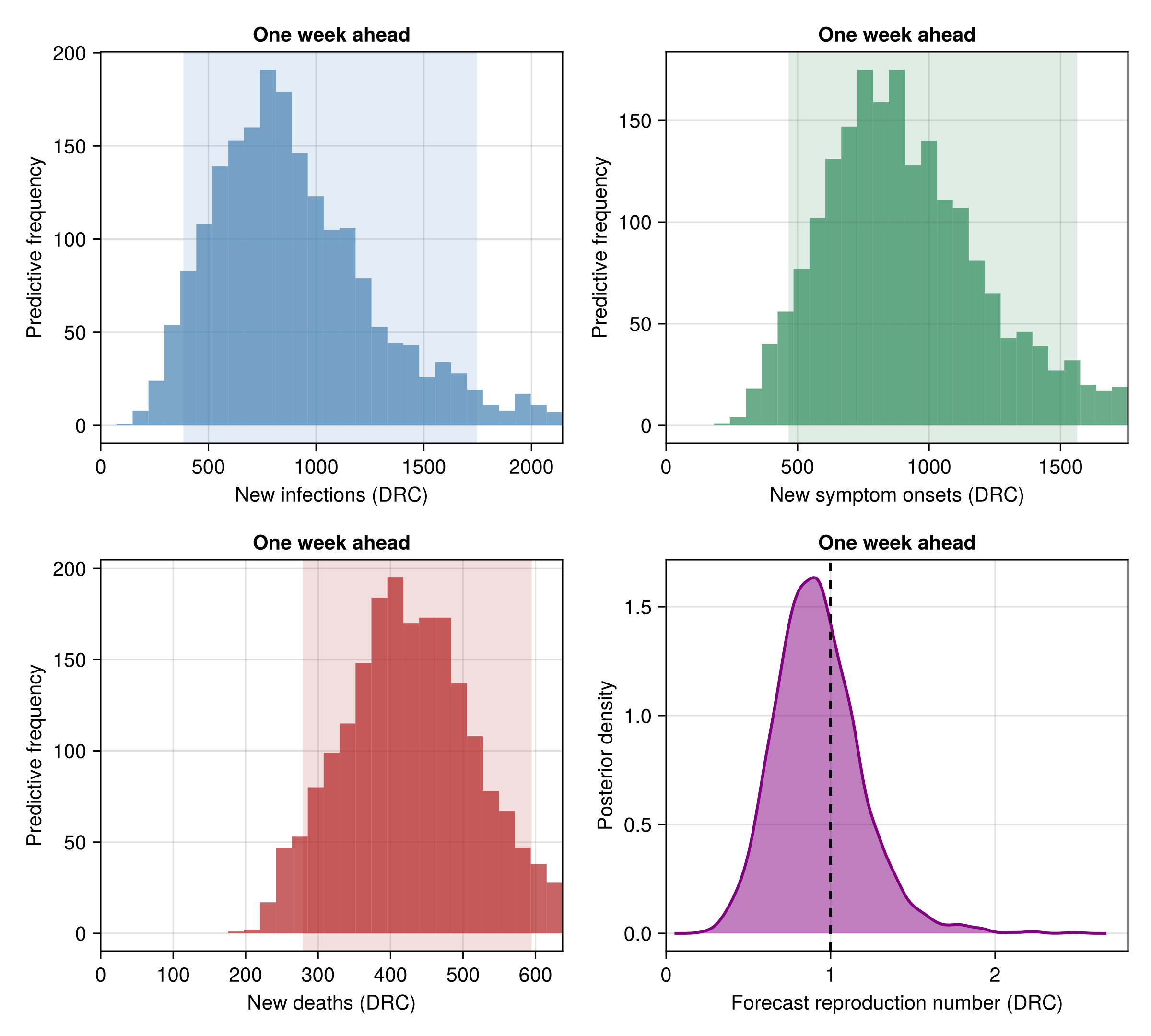
The observed figure shows the new count each observed stream adds over the horizon: suspected cases, suspected deaths, laboratory-confirmed cases, confirmed deaths and recovered, one panel per stream the forecast carries.
One-week-ahead observed forecast plot
forecast_fig = plot_forecast(forecast);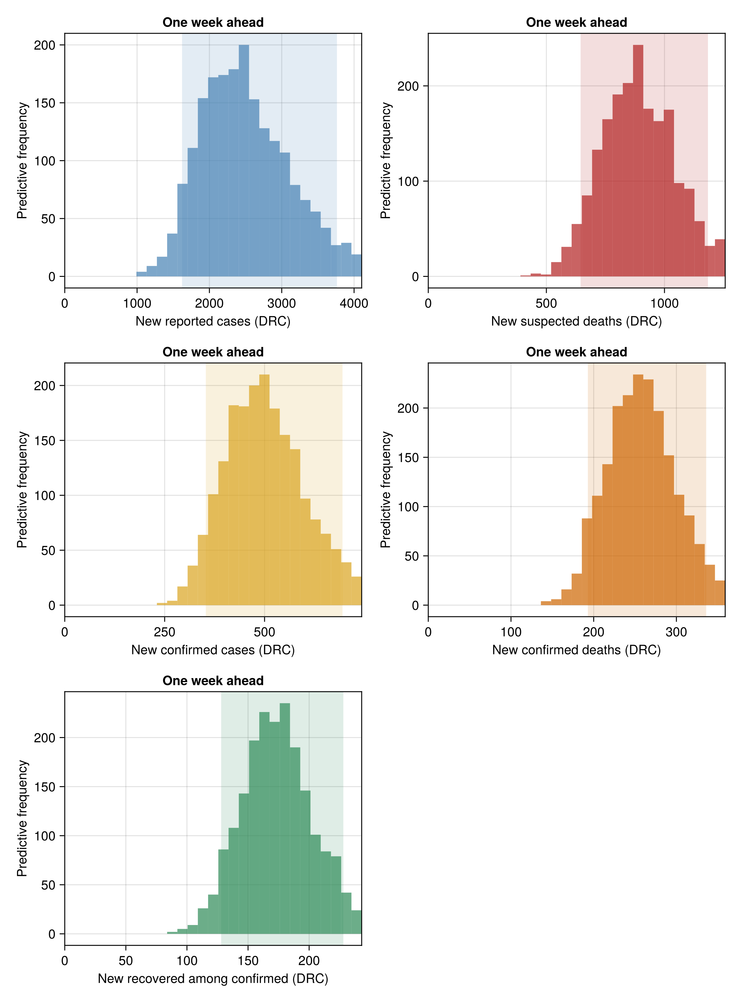
The bed figure shows the projected isolation/treatment-bed demand (the need a week ahead, under unconstrained supply) against the supply-limited occupancy the beds can actually meet. The gap between the two is the projected bed shortfall, shown in the right panel. The reported "Patients en isolement" count is the occupied-bed count (the report computes the "Taux d'occupation" as that count over the bed capacity), so isolation is bed usage, gated by supply. The demand is its unobserved counterpart, the number who need a bed. The model carries a single national bed capacity, so it cannot represent local saturation, and the national shortfall understates local unmet need. On 13 June Ituri was at 93.9% occupancy while Sud-Kivu was at 21.9%; beds free in one province cannot serve patients in another.
One-week-ahead isolation-bed forecast plot
forecast_beds_fig = plot_forecast_beds(forecast);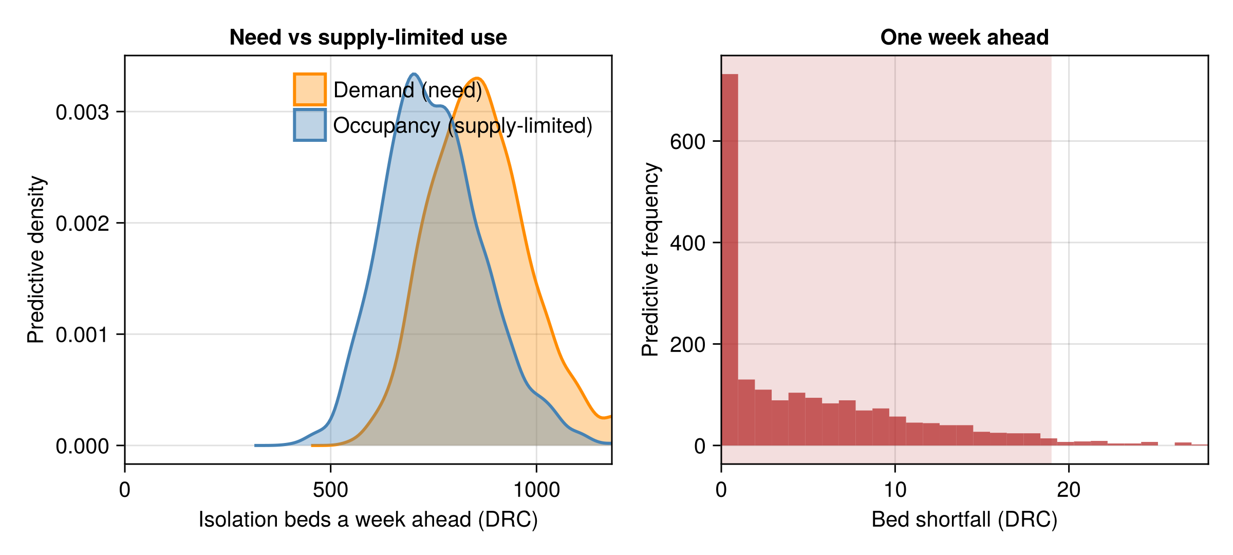
The flow figure projects the daily isolation/treatment flows a week ahead: new admissions, in-care deaths and rule-outs, each drawn from the model run past the cut-off through the isolation dispersion.
One-week-ahead treatment-flow forecast plot
forecast_flows_fig = plot_forecast_flows(forecast);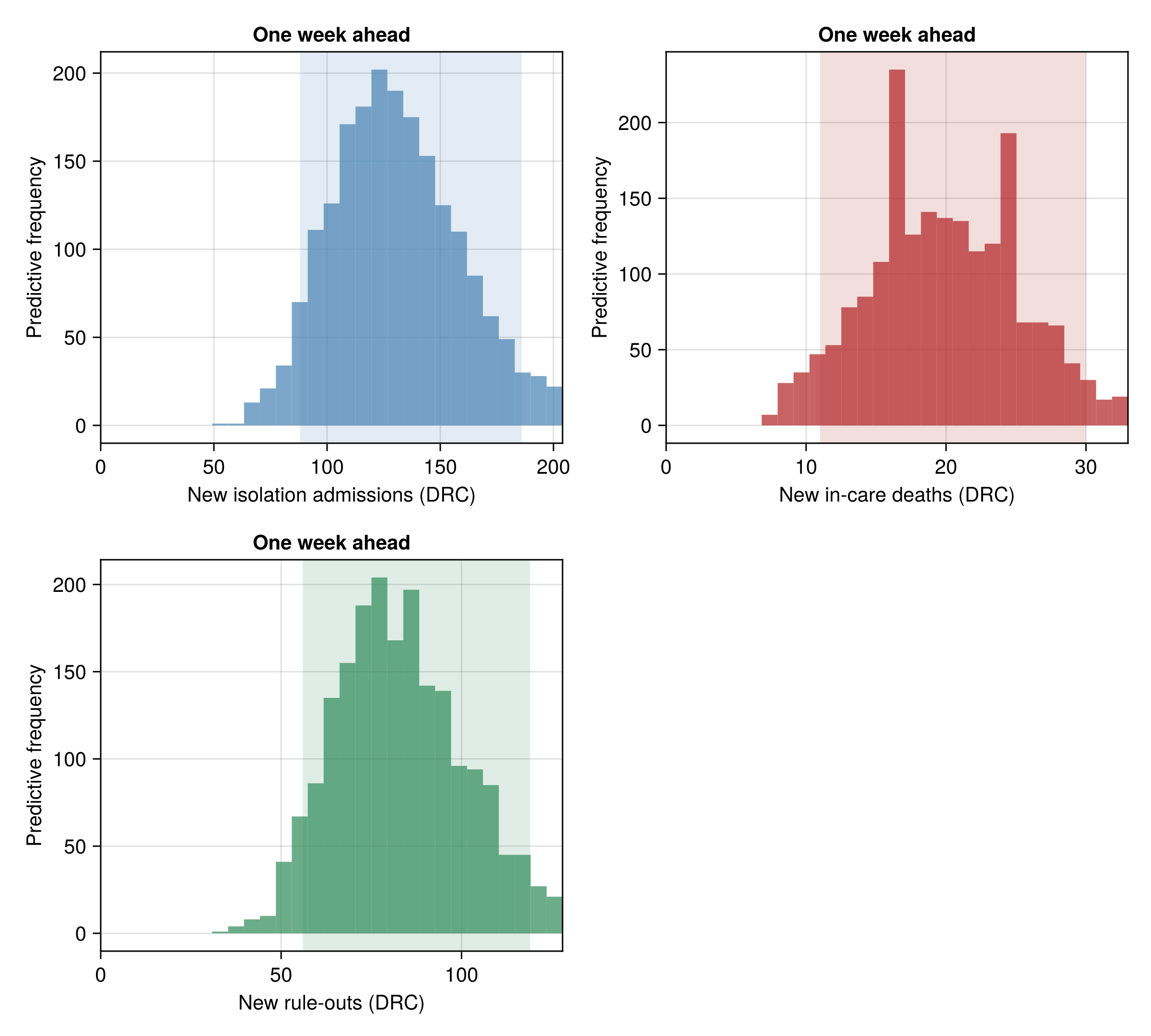
Symptom-onset nowcast and forecast results
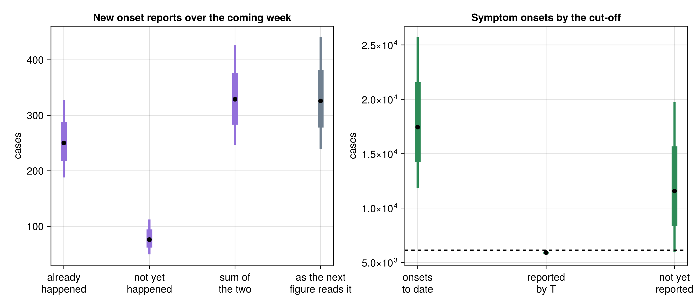
The table below gives the onset stream's projection, built as described in the symptom-onset nowcast and forecast Methods section. The two halves must not be added together: the first three rows are the state of the outbreak at the cut-off, the next three the coming week.
"Onsets not yet reported at T" is not a backlog that will all arrive, because ascertainment does not reach one. The row holds two things together: the reporting backlog, and the cases surveillance will never confirm. The "reports this week of onsets before T" row is the part of it the coming week should actually clear. It is the smaller number.
Generate the symptom-onset nowcast and forecast
onset_forecast = forecast_onsets(
    fit_forecast("joint");
    horizon = 7,
    obs_value = something(obs.onset_curve_history.last_total, 0)
);
onset_forecast_summary = onset_forecast_table(onset_forecast);
Symptom-onset nowcast and forecast summary table
| Row | Quantity | Lower 90% | Lower 60% | Lower 30% | Upper 30% | Upper 60% | Upper 90% |
|---|---|---|---|---|---|---|---|
| String | Float64 | Float64 | Float64 | Float64 | Float64 | Float64 | |
| 1 | symptom onsets to date | 11845.0 | 14233.0 | 15853.0 | 19353.0 | 21569.0 | 25724.0 |
| 2 | of those, reported by T | 5742.0 | 5812.0 | 5858.0 | 5933.0 | 5978.0 | 6060.0 |
| 3 | onsets not yet reported at T | 5973.0 | 8361.0 | 9955.0 | 13445.0 | 15673.0 | 19738.0 |
| 4 | reports this week of onsets before T | 188.0 | 218.0 | 235.0 | 266.0 | 288.0 | 328.0 |
| 5 | reports this week of onsets after T | 50.0 | 62.0 | 69.0 | 84.0 | 94.0 | 112.0 |
| 6 | new onset reports this week | 239.0 | 278.0 | 304.0 | 351.0 | 382.0 | 441.0 |
| 7 | new symptom onsets this week | 466.0 | 656.0 | 775.0 | 1000.0 | 1170.0 | 1563.0 |
The left panel splits the coming week's new onset reports into reports of onsets that had already happened by the cut-off and reports of onsets still to come, and shows their sum. The fourth bar is the same sum after it has been through the observation model, which is what the next vintage will actually print. It is wider than the sum it replicates by the two reads' error and the counting variation of the new reports. Only the fourth bar is comparable to a digitised figure, and only it is scored.
The right panel puts the nowcast itself on the same axes, the onsets that have happened against the share of them the triangle has printed.
Symptom-onset nowcast and forecast plot
onset_forecast_fig = let
    fig = CairoMakie.Figure(; size = (960, 420))
    # Two-line tick labels rather than rotated ones: the leftmost rotated
    # label overhangs the axis and is clipped at the figure edge.
    ax1 = CairoMakie.Axis(
        fig[1, 1];
        title = "New onset reports over the coming week",
        ylabel = "cases", xticks = (
            1:4,
            [
                "already\nhappened", "not yet\nhappened", "sum of\nthe two",
                "as the next\nfigure reads it",
            ],
        )
    )
    # The first three bars are latent, so the third is exactly the first
    # two added. The fourth is that same sum replicated through the
    # observation model, which is the scored quantity and the only one
    # comparable to a digitised figure; it is wider by the read error,
    # which is why the three latent bars are shown as well rather than a
    # decomposition that appears not to add up.
    _latent_total = onset_forecast.onset_reports_backfill .+
        onset_forecast.onset_reports_future
    for (i, d, col) in (
            (
                1, onset_forecast.onset_reports_backfill,
                :mediumpurple,
            ),
            (2, onset_forecast.onset_reports_future, :mediumpurple),
            (3, _latent_total, :mediumpurple),
            (4, Float64.(onset_forecast.onset_reports_new), :slategray),
        )
        s = posterior_summary(d)
        CairoMakie.rangebars!(
            ax1, [Float64(i)], [s.lo90], [s.hi90];
            color = col, linewidth = 3
        )
        CairoMakie.rangebars!(
            ax1, [Float64(i)], [s.lo60], [s.hi60];
            color = col, linewidth = 8
        )
        CairoMakie.scatter!(
            ax1, [Float64(i)], [quantile(d, 0.5)];
            color = :black, markersize = 9
        )
    end
    ax2 = CairoMakie.Axis(
        fig[1, 2];
        title = "Symptom onsets by the cut-off",
        ylabel = "cases", xticks = (
            1:3,
            ["onsets\nto date", "reported\nby T", "not yet\nreported"],
        )
    )
    for (i, d) in enumerate(
            (
                onset_forecast.onsets_to_date,
                onset_forecast.onset_reports_to_date,
                onset_forecast.onsets_unreported,
            )
        )
        s = posterior_summary(d)
        CairoMakie.rangebars!(
            ax2, [Float64(i)], [s.lo90], [s.hi90];
            color = :seagreen, linewidth = 3
        )
        CairoMakie.rangebars!(
            ax2, [Float64(i)], [s.lo60], [s.hi60];
            color = :seagreen, linewidth = 8
        )
        CairoMakie.scatter!(
            ax2, [Float64(i)], [quantile(d, 0.5)];
            color = :black, markersize = 9
        )
    end
    # The digitised total the "reported by T" bar is a model of, so the
    # reader can see the fitted reported level against the figure itself.
    ismissing(obs.onset_curve_history.last_total) ||
        CairoMakie.hlines!(
        ax2,
        [Float64(obs.onset_curve_history.last_total)];
        color = :black, linestyle = :dash
    )
    fig
end;