The scoringutils package provides a collection of
metrics and proper scoring rules that make it simple to score
probabilistic forecasts against the true observed values. You can find
more information in the paper Evaluating Forecasts with
scoringutils in R as well as the Metrics-Vignette
and the Scoring
forecasts directly Vignette.
The scoringutils package offers convenient automated
forecast evaluation in a data.table format (using the
function score()), but also provides experienced users with
a set of reliable lower-level scoring metrics operating on
vectors/matriced they can build upon in other applications. In addition
it implements a wide range of flexible plots that are able to cover many
use cases.
The goal of this package is to provide a tested and reliable
collection of metrics that can be used for scoring probabilistic
forecasts (forecasts with a full predictive distribution, rather than
point forecasts). It has a much stronger focus on convenience than
e.g. the scoringRules package, which provides a
comprehensive collection of proper scoring rules (also used in
scoringutils). In contrast to other packages,
scoringutils offers functionality to automatically evaluate
forecasts, to visualise scores and to obtain relative scores between
models.
Predictions can be handled in various formats:
scoringutils can handle probabilistic forecasts in either a
sample based or a quantile based format. For more detail on the expected
input formats please see below. True values can be integer, continuous
or binary.
Input formats
Most of the time, the score() function will be able to
do the entire evaluation for you. All you need to do is to pass in a
data.frame with the appropriate columns. Which columns are
required depends on the format the forecasts come in. The forecast
format can either be based on quantiles (see
example_quantile for the expected format), based on
predictive samples (see example_continuous and
example_integer for the expected format in each case) or in
a binary format. The following table gives an overview (pairwise
comparisons will be explained in more detail below):
| Format | Required columns |
|---|---|
| quantile-based | ‘true_value’, ‘prediction’, ‘quantile’ |
| sample-based | ‘true_value’, ‘prediction’, ‘sample’ |
| binary | ‘true_value’, ‘prediction’ |
| pairwise-comparisons | additionally a column ‘model’ |
Additional columns may be present to indicate a grouping of
forecasts. For example, we could have forecasts made by different models
in various locations at different time points, each for several weeks
into the future. scoringutils automatically tries to
determine the unit of a single forecast, i.e. the combination
of existing columns that are able to uniquely identify a single
forecast. It uses all existing columns for this, which can sometimes
lead to issues. We therefore recommend using the function
set_forecast_unit() to determine the forecast unit
manually. The function simply drops unneeded columns, while making sure
that some necessary, ‘protected columns’ like “prediction” or
“true_value” are retained.
colnames(example_quantile)
#>  [1] "location"        "target_end_date" "target_type"     "true_value"
#>  [5] "location_name"   "forecast_date"   "quantile"        "prediction"
#>  [9] "model"           "horizon"

set_forecast_unit(
  example_quantile,
  c("location", "target_end_date", "target_type", "horizon", "model")
) %>%
  colnames()
#> [1] "true_value"      "quantile"        "prediction"      "location"
#> [5] "target_end_date" "target_type"     "horizon"         "model"
Checking the input data
The function check_forecasts() can be used to check the
input data. It gives a summary of what scoringutils thinks
you are trying to achieve. It infers the type of the prediction target,
the prediction format, and the unit of a single forecasts, gives an
overview of the number of unique values per column (helpful for spotting
missing data) and returns warnings or errors.
head(example_quantile)
#>    location target_end_date target_type true_value location_name forecast_date
#> 1:       DE      2021-01-02       Cases     127300       Germany          <NA>
#> 2:       DE      2021-01-02      Deaths       4534       Germany          <NA>
#> 3:       DE      2021-01-09       Cases     154922       Germany          <NA>
#> 4:       DE      2021-01-09      Deaths       6117       Germany          <NA>
#> 5:       DE      2021-01-16       Cases     110183       Germany          <NA>
#> 6:       DE      2021-01-16      Deaths       5867       Germany          <NA>
#>    quantile prediction model horizon
#> 1:       NA         NA  <NA>      NA
#> 2:       NA         NA  <NA>      NA
#> 3:       NA         NA  <NA>      NA
#> 4:       NA         NA  <NA>      NA
#> 5:       NA         NA  <NA>      NA
#> 6:       NA         NA  <NA>      NA
check_forecasts(example_quantile)
#> The following messages were produced when checking inputs:
#> 1.  144 values for `prediction` are NA in the data provided and the corresponding rows were removed. This may indicate a problem if unexpected.
#> Your forecasts seem to be for a target of the following type:
#> $target_type
#> [1] "integer"
#>
#> and in the following format:
#> $prediction_type
#> [1] "quantile"
#>
#> The unit of a single forecast is defined by:
#> $forecast_unit
#> [1] "location"        "target_end_date" "target_type"     "location_name"
#> [5] "forecast_date"   "model"           "horizon"
#>
#> Cleaned data, rows with NA values in prediction or true_value removed:
#> $cleaned_data
#>        location target_end_date target_type true_value location_name
#>     1:       DE      2021-05-08       Cases     106987       Germany
#>     2:       DE      2021-05-08       Cases     106987       Germany
#>     3:       DE      2021-05-08       Cases     106987       Germany
#>     4:       DE      2021-05-08       Cases     106987       Germany
#>     5:       DE      2021-05-08       Cases     106987       Germany
#>    ---
#> 20397:       IT      2021-07-24      Deaths         78         Italy
#> 20398:       IT      2021-07-24      Deaths         78         Italy
#> 20399:       IT      2021-07-24      Deaths         78         Italy
#> 20400:       IT      2021-07-24      Deaths         78         Italy
#> 20401:       IT      2021-07-24      Deaths         78         Italy
#>        forecast_date quantile prediction                 model horizon
#>     1:    2021-05-03    0.010      82466 EuroCOVIDhub-ensemble       1
#>     2:    2021-05-03    0.025      86669 EuroCOVIDhub-ensemble       1
#>     3:    2021-05-03    0.050      90285 EuroCOVIDhub-ensemble       1
#>     4:    2021-05-03    0.100      95341 EuroCOVIDhub-ensemble       1
#>     5:    2021-05-03    0.150      99171 EuroCOVIDhub-ensemble       1
#>    ---
#> 20397:    2021-07-12    0.850        352  epiforecasts-EpiNow2       2
#> 20398:    2021-07-12    0.900        397  epiforecasts-EpiNow2       2
#> 20399:    2021-07-12    0.950        499  epiforecasts-EpiNow2       2
#> 20400:    2021-07-12    0.975        611  epiforecasts-EpiNow2       2
#> 20401:    2021-07-12    0.990        719  epiforecasts-EpiNow2       2
#>
#> Number of unique values per column per model:
#> $unique_values
#>                    model location target_end_date target_type true_value
#> 1: EuroCOVIDhub-ensemble        4              12           2         96
#> 2: EuroCOVIDhub-baseline        4              12           2         96
#> 3:  epiforecasts-EpiNow2        4              12           2         95
#> 4:       UMass-MechBayes        4              12           1         48
#>    location_name forecast_date quantile prediction horizon
#> 1:             4            11       23       3969       3
#> 2:             4            11       23       3733       3
#> 3:             4            11       23       3903       3
#> 4:             4            11       23       1058       3
#>
#> $messages
#> [1] "144 values for `prediction` are NA in the data provided and the corresponding rows were removed. This may indicate a problem if unexpected."
If you are unsure what your input data should look like, have a look
at the example_quantile, example_integer,
example_continuous and example_binary data
sets provided in the package.
The output of check_forecasts() can later be directly
used as input to score() (otherwise, score()
will just run check_forecasts() anyway internally).
Showing available forecasts
The function avail_forecasts() may also be helpful to
determine where forecasts are available. Using the by
argument you can specify the level of summary. For example, to see how
many forecasts there are per model and target_type, we can run
avail_forecasts(example_quantile, by = c("model", "target_type"))
#> The following messages were produced when checking inputs:
#> 1.  144 values for `prediction` are NA in the data provided and the corresponding rows were removed. This may indicate a problem if unexpected.
#>                    model target_type Number forecasts
#> 1: EuroCOVIDhub-ensemble       Cases              128
#> 2: EuroCOVIDhub-baseline       Cases              128
#> 3:  epiforecasts-EpiNow2       Cases              128
#> 4: EuroCOVIDhub-ensemble      Deaths              128
#> 5: EuroCOVIDhub-baseline      Deaths              128
#> 6:       UMass-MechBayes      Deaths              128
#> 7:  epiforecasts-EpiNow2      Deaths              119
We see that ‘epiforecasts-EpiNow2’ has some missing forecasts for the deaths forecast target and that UMass-MechBayes has no case forecasts.
This information can also be visualised using the
plot_avail_forecasts() function:
example_quantile %>%
  avail_forecasts(by = c("model", "forecast_date", "target_type")) %>%
  plot_avail_forecasts() +
  facet_wrap(~ target_type)
#> The following messages were produced when checking inputs:
#> 1.  144 values for `prediction` are NA in the data provided and the corresponding rows were removed. This may indicate a problem if unexpected.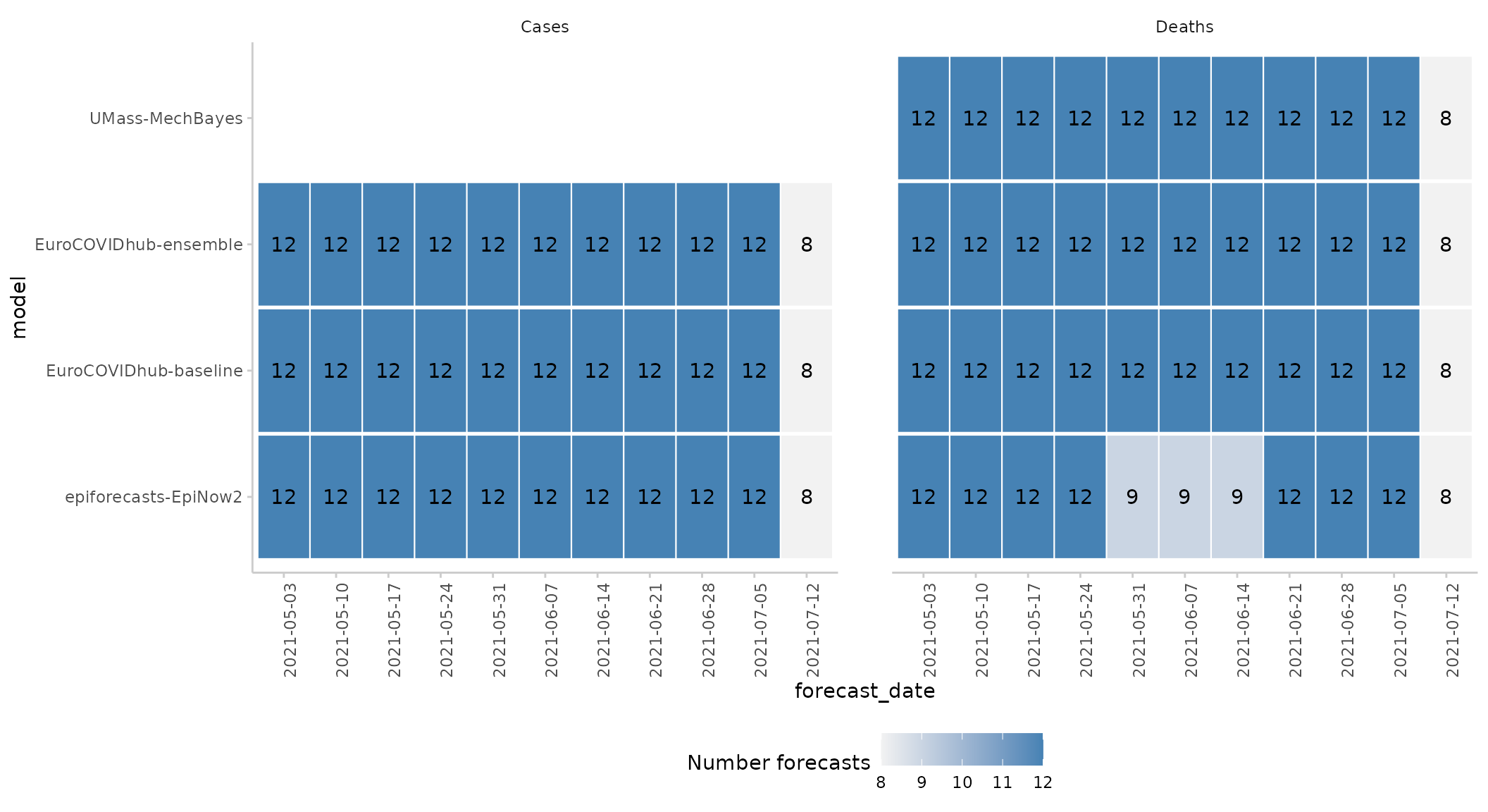
You can also visualise forecasts directly using the
plot_predictions() function:
example_quantile %>%
  make_NA(
    what = "truth",
    target_end_date >= "2021-07-15",
    target_end_date < "2021-05-22"
  ) %>%
  make_NA(
    what = "forecast",
    model != "EuroCOVIDhub-ensemble",
    forecast_date != "2021-06-28"
  ) %>%
  plot_predictions(
    x = "target_end_date",
    by = c("target_type", "location")
  ) +
  facet_wrap(target_type ~ location, ncol = 4, scales = "free")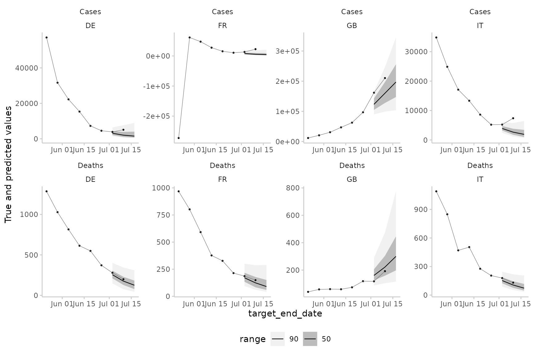
Scoring and summarising forecasts
Forecasts can easily be scored using the score()
function.
For clarity, we suggest setting the forecast unit explicitly and you
may also want to call check_forecasts() explicitly.
scores <- example_quantile %>%
  set_forecast_unit(
    c("location", "target_end_date", "target_type", "location_name",
      "forecast_date", "model", "horizon")
  ) %>%
  check_forecasts() %>%
  score()
#> The following messages were produced when checking inputs:
#> 1.  144 values for `prediction` are NA in the data provided and the corresponding rows were removed. This may indicate a problem if unexpected.
head(scores)
#>    location target_end_date target_type location_name forecast_date
#> 1:       DE      2021-05-08       Cases       Germany    2021-05-03
#> 2:       DE      2021-05-08       Cases       Germany    2021-05-03
#> 3:       DE      2021-05-08       Cases       Germany    2021-05-03
#> 4:       DE      2021-05-08       Cases       Germany    2021-05-03
#> 5:       DE      2021-05-08       Cases       Germany    2021-05-03
#> 6:       DE      2021-05-08       Cases       Germany    2021-05-03
#>                    model horizon range interval_score dispersion
#> 1: EuroCOVIDhub-baseline       1     0        25620.0        0.0
#> 2: EuroCOVIDhub-baseline       1    10        25599.5      184.5
#> 3: EuroCOVIDhub-baseline       1    10        25599.5      184.5
#> 4: EuroCOVIDhub-baseline       1    20        25481.0      556.0
#> 5: EuroCOVIDhub-baseline       1    20        25481.0      556.0
#> 6: EuroCOVIDhub-baseline       1    30        25270.2      816.2
#>    underprediction overprediction coverage coverage_deviation bias quantile
#> 1:               0          25620        0                0.0 0.95     0.50
#> 2:               0          25415        0               -0.1 0.95     0.45
#> 3:               0          25415        0               -0.1 0.95     0.55
#> 4:               0          24925        0               -0.2 0.95     0.40
#> 5:               0          24925        0               -0.2 0.95     0.60
#> 6:               0          24454        0               -0.3 0.95     0.35
#>    ae_median quantile_coverage
#> 1:     25620              TRUE
#> 2:     25620              TRUE
#> 3:     25620              TRUE
#> 4:     25620              TRUE
#> 5:     25620              TRUE
#> 6:     25620              TRUE
Note that in the above example some columns contain duplicated information with regards to the forecast unit, e.g. “location” and “location_name”, and could be dropped.
example_quantile %>%
  set_forecast_unit(
    c("location", "target_end_date", "target_type",
      "forecast_date", "model", "horizon")
  ) %>%
  check_forecasts()
#> The following messages were produced when checking inputs:
#> 1.  144 values for `prediction` are NA in the data provided and the corresponding rows were removed. This may indicate a problem if unexpected.
#> Your forecasts seem to be for a target of the following type:
#> $target_type
#> [1] "integer"
#>
#> and in the following format:
#> $prediction_type
#> [1] "quantile"
#>
#> The unit of a single forecast is defined by:
#> $forecast_unit
#> [1] "location"        "target_end_date" "target_type"     "forecast_date"
#> [5] "model"           "horizon"
#>
#> Cleaned data, rows with NA values in prediction or true_value removed:
#> $cleaned_data
#>        true_value quantile prediction location target_end_date target_type
#>     1:     106987    0.010      82466       DE      2021-05-08       Cases
#>     2:     106987    0.025      86669       DE      2021-05-08       Cases
#>     3:     106987    0.050      90285       DE      2021-05-08       Cases
#>     4:     106987    0.100      95341       DE      2021-05-08       Cases
#>     5:     106987    0.150      99171       DE      2021-05-08       Cases
#>    ---
#> 20397:         78    0.850        352       IT      2021-07-24      Deaths
#> 20398:         78    0.900        397       IT      2021-07-24      Deaths
#> 20399:         78    0.950        499       IT      2021-07-24      Deaths
#> 20400:         78    0.975        611       IT      2021-07-24      Deaths
#> 20401:         78    0.990        719       IT      2021-07-24      Deaths
#>        forecast_date                 model horizon
#>     1:    2021-05-03 EuroCOVIDhub-ensemble       1
#>     2:    2021-05-03 EuroCOVIDhub-ensemble       1
#>     3:    2021-05-03 EuroCOVIDhub-ensemble       1
#>     4:    2021-05-03 EuroCOVIDhub-ensemble       1
#>     5:    2021-05-03 EuroCOVIDhub-ensemble       1
#>    ---
#> 20397:    2021-07-12  epiforecasts-EpiNow2       2
#> 20398:    2021-07-12  epiforecasts-EpiNow2       2
#> 20399:    2021-07-12  epiforecasts-EpiNow2       2
#> 20400:    2021-07-12  epiforecasts-EpiNow2       2
#> 20401:    2021-07-12  epiforecasts-EpiNow2       2
#>
#> Number of unique values per column per model:
#> $unique_values
#>                    model true_value quantile prediction location
#> 1: EuroCOVIDhub-ensemble         96       23       3969        4
#> 2: EuroCOVIDhub-baseline         96       23       3733        4
#> 3:  epiforecasts-EpiNow2         95       23       3903        4
#> 4:       UMass-MechBayes         48       23       1058        4
#>    target_end_date target_type forecast_date horizon
#> 1:              12           2            11       3
#> 2:              12           2            11       3
#> 3:              12           2            11       3
#> 4:              12           1            11       3
#>
#> $messages
#> [1] "144 values for `prediction` are NA in the data provided and the corresponding rows were removed. This may indicate a problem if unexpected."
If we drop essential information, for example, the “target_type” column, we’ll get an error informing us that the forecasts aren’t uniquely identified any more.
example_quantile %>%
  set_forecast_unit(
    c("location", "target_end_date",
      "forecast_date", "model", "horizon")
  ) %>%
  check_forecasts()
#> The following messages were produced when checking inputs:
#> 1.  144 values for `prediction` are NA in the data provided and the corresponding rows were removed. This may indicate a problem if unexpected.
#> Warning in check_forecasts(.): The following warnings were produced when checking inputs:
#> 1.  Some forecasts have different numbers of rows
#> 2.  (e.g. quantiles or samples).
#> 3.  scoringutils found:
#> 4.  46, 23
#> 5.  . This may be a problem (it can potentially distort scores,
#> 6.  making it more difficult to compare them),
#> 7.  so make sure this is intended.
#> Error in check_forecasts(.): The following errors were produced when checking inputs:
#> 1.  There are instances with more than one forecast for the same target. This can't be right and needs to be resolved. Maybe you need to check the unit of a single forecast and add missing columns? Use the  function find_duplicates() to identify duplicate rows.
The function find_duplicates() may help to investigate
the issue. When filtering for only median forecasts of the
EuroCOVIDhub-ensemble, we can see that there are indeed two forecasts
for every date, location and horizon.
duplicates <- example_quantile %>%
  set_forecast_unit(
    c("location", "target_end_date",
      "forecast_date", "model", "horizon")
  ) %>%
  find_duplicates()

duplicates[quantile == 0.5 & model == "EuroCOVIDhub-ensemble", ] %>%
  head()
#>    true_value quantile prediction location target_end_date forecast_date
#> 1:     106987      0.5     119258       DE      2021-05-08    2021-05-03
#> 2:       1582      0.5       1568       DE      2021-05-08    2021-05-03
#> 3:      64985      0.5     110716       DE      2021-05-15    2021-05-03
#> 4:      64985      0.5      92649       DE      2021-05-15    2021-05-10
#> 5:       1311      0.5       1521       DE      2021-05-15    2021-05-03
#> 6:       1311      0.5       1422       DE      2021-05-15    2021-05-10
#>                    model horizon
#> 1: EuroCOVIDhub-ensemble       1
#> 2: EuroCOVIDhub-ensemble       1
#> 3: EuroCOVIDhub-ensemble       2
#> 4: EuroCOVIDhub-ensemble       1
#> 5: EuroCOVIDhub-ensemble       2
#> 6: EuroCOVIDhub-ensemble       1
The function score() returns unsumarised scores, which
in most cases is not what the user wants. It returns a single score per
forecast (as determined by the forecast unit). For forecasts in a
quantile format, it returns one score per quantile.
A second function, summarise_scores() takes care of
summarising these scores to the level specified by the user. The
by argument can be used to define the level of summary. By
default, by = NULL and the summary unit is assumed to be
the same as the unit of a single forecast. For continuous forecasts,
this means that nothing happens if by isn’t specified.
scores <- score(example_continuous)
#> The following messages were produced when checking inputs:
#> 1.  144 values for `prediction` are NA in the data provided and the corresponding rows were removed. This may indicate a problem if unexpected.
all(scores == summarise_scores(scores), na.rm = TRUE)
#> [1] TRUE
For quantile based forecasts, if by = NULL, then scores
are summarised across quantiles and instead of one score per
forecast_unit and quantile we only get one score per forecast unit.
scores <- example_quantile %>%
  set_forecast_unit(
    c("location", "target_end_date", "target_type",
      "forecast_date", "model", "horizon")
  ) %>%
  check_forecasts() %>%
  score()
#> The following messages were produced when checking inputs:
#> 1.  144 values for `prediction` are NA in the data provided and the corresponding rows were removed. This may indicate a problem if unexpected.

head(scores)
#>    location target_end_date target_type forecast_date                 model
#> 1:       DE      2021-05-08       Cases    2021-05-03 EuroCOVIDhub-baseline
#> 2:       DE      2021-05-08       Cases    2021-05-03 EuroCOVIDhub-baseline
#> 3:       DE      2021-05-08       Cases    2021-05-03 EuroCOVIDhub-baseline
#> 4:       DE      2021-05-08       Cases    2021-05-03 EuroCOVIDhub-baseline
#> 5:       DE      2021-05-08       Cases    2021-05-03 EuroCOVIDhub-baseline
#> 6:       DE      2021-05-08       Cases    2021-05-03 EuroCOVIDhub-baseline
#>    horizon range interval_score dispersion underprediction overprediction
#> 1:       1     0        25620.0        0.0               0          25620
#> 2:       1    10        25599.5      184.5               0          25415
#> 3:       1    10        25599.5      184.5               0          25415
#> 4:       1    20        25481.0      556.0               0          24925
#> 5:       1    20        25481.0      556.0               0          24925
#> 6:       1    30        25270.2      816.2               0          24454
#>    coverage coverage_deviation bias quantile ae_median quantile_coverage
#> 1:        0                0.0 0.95     0.50     25620              TRUE
#> 2:        0               -0.1 0.95     0.45     25620              TRUE
#> 3:        0               -0.1 0.95     0.55     25620              TRUE
#> 4:        0               -0.2 0.95     0.40     25620              TRUE
#> 5:        0               -0.2 0.95     0.60     25620              TRUE
#> 6:        0               -0.3 0.95     0.35     25620              TRUE

scores %>%
  summarise_scores() %>%
  head()
#>    location target_end_date target_type forecast_date                 model
#> 1:       DE      2021-05-08       Cases    2021-05-03 EuroCOVIDhub-baseline
#> 2:       DE      2021-05-08       Cases    2021-05-03 EuroCOVIDhub-ensemble
#> 3:       DE      2021-05-08       Cases    2021-05-03  epiforecasts-EpiNow2
#> 4:       DE      2021-05-08      Deaths    2021-05-03 EuroCOVIDhub-baseline
#> 5:       DE      2021-05-08      Deaths    2021-05-03 EuroCOVIDhub-ensemble
#> 6:       DE      2021-05-08      Deaths    2021-05-03       UMass-MechBayes
#>    horizon interval_score dispersion underprediction overprediction
#> 1:       1    16925.04696 1649.22087       0.0000000   15275.826087
#> 2:       1     7990.85478 5440.98522       0.0000000    2549.869565
#> 3:       1    25395.96087 8173.70000       0.0000000   17222.260870
#> 4:       1       46.79304   44.66261       0.0000000       2.130435
#> 5:       1       53.88000   53.27130       0.6086957       0.000000
#> 6:       1      116.12174   77.07826      39.0434783       0.000000
#>    coverage_deviation  bias ae_median
#> 1:        -0.38521739  0.95     25620
#> 2:         0.04956522  0.50     12271
#> 3:        -0.29826087  0.90     44192
#> 4:         0.22347826  0.30        15
#> 5:         0.39739130 -0.10        14
#> 6:         0.04956522 -0.50       208
Through the by argument we can specify what unit of
summary we want. We can also call sumarise_scores()
multiple tines, e.g to round your outputs by specifying
e.g. signif() as a summary function.
scores %>%
  summarise_scores(by = c("model", "target_type")) %>%
  summarise_scores(fun = signif, digits = 2) %>%
kable()| model | target_type | interval_score | dispersion | underprediction | overprediction | coverage_deviation | bias | ae_median |
|---|---|---|---|---|---|---|---|---|
| EuroCOVIDhub-baseline | Cases | 28000 | 4100 | 10000.0 | 14000.0 | -0.110 | 0.0980 | 38000 |
| EuroCOVIDhub-ensemble | Cases | 18000 | 3700 | 4200.0 | 10000.0 | -0.098 | -0.0560 | 24000 |
| epiforecasts-EpiNow2 | Cases | 21000 | 5700 | 3300.0 | 12000.0 | -0.067 | -0.0790 | 28000 |
| EuroCOVIDhub-baseline | Deaths | 160 | 91 | 2.1 | 66.0 | 0.120 | 0.3400 | 230 |
| EuroCOVIDhub-ensemble | Deaths | 41 | 30 | 4.1 | 7.1 | 0.200 | 0.0730 | 53 |
| UMass-MechBayes | Deaths | 53 | 27 | 17.0 | 9.0 | -0.023 | -0.0220 | 78 |
| epiforecasts-EpiNow2 | Deaths | 67 | 32 | 16.0 | 19.0 | -0.043 | -0.0051 | 100 |
Scoring point forecasts
Point forecasts can be scored by making use of the quantile-based
format, but with a value of NA or "point" in
the quantile column. Point forecasts can be scored alongside other
quantile-based forecasts. As point forecasts will have values of
NA for metrics designed for probabilistic forecasts, it is
important to use na.rm = TRUE when summarising.
suppressMessages(score(example_point)) %>%
  summarise_scores(by = "model", na.rm = TRUE)
#>                    model interval_score dispersion underprediction
#> 1: EuroCOVIDhub-baseline     14092.7647 2192.26967      4996.92898
#> 2: EuroCOVIDhub-ensemble      8852.4196 1930.80064      2005.56357
#> 3:  epiforecasts-EpiNow2     10659.5125 3084.85850      1604.96135
#> 4:       UMass-MechBayes        51.4781   28.09387        15.32315
#>    overprediction coverage_deviation        bias    ae_point     se_point
#> 1:     6903.56605        0.002102273  0.21851562 19353.42969 2.883446e+09
#> 2:     4916.05540        0.050752841  0.00812500 12077.10156 1.945118e+09
#> 3:     5969.69268       -0.057861612 -0.04376518 14521.10526 2.680928e+09
#> 4:        8.06108       -0.024886364 -0.02312500    78.47656 1.170976e+04
#>    ae_median
#> 1:       NaN
#> 2:       NaN
#> 3:       NaN
#> 4:       NaN
Adding empirical coverage
For quantile-based forecasts we are often interested in specific
coverage-levels, for example, what percentage of true values fell
between all 50% or the 90% prediction intervals. We can add this
information using the function add_coverage(). This
function also requires a by argument which defines the
level of grouping for which the percentage of true values covered by
certain prediction intervals is computed.
score(example_quantile) %>%
  add_coverage(ranges = c(50, 90), by = c("model", "target_type")) %>%
  summarise_scores(by = c("model", "target_type")) %>%
  summarise_scores(fun = signif, digits = 2)
#> The following messages were produced when checking inputs:
#> 1.  144 values for `prediction` are NA in the data provided and the corresponding rows were removed. This may indicate a problem if unexpected.
#>                    model target_type interval_score dispersion underprediction
#> 1: EuroCOVIDhub-baseline       Cases          28000       4100         10000.0
#> 2: EuroCOVIDhub-baseline      Deaths            160         91             2.1
#> 3: EuroCOVIDhub-ensemble       Cases          18000       3700          4200.0
#> 4: EuroCOVIDhub-ensemble      Deaths             41         30             4.1
#> 5:       UMass-MechBayes      Deaths             53         27            17.0
#> 6:  epiforecasts-EpiNow2       Cases          21000       5700          3300.0
#> 7:  epiforecasts-EpiNow2      Deaths             67         32            16.0
#>    overprediction coverage_deviation    bias ae_median coverage_50 coverage_90
#> 1:        14000.0             -0.110  0.0980     38000        0.33        0.82
#> 2:           66.0              0.120  0.3400       230        0.66        1.00
#> 3:        10000.0             -0.098 -0.0560     24000        0.39        0.80
#> 4:            7.1              0.200  0.0730        53        0.88        1.00
#> 5:            9.0             -0.023 -0.0220        78        0.46        0.88
#> 6:        12000.0             -0.067 -0.0790     28000        0.47        0.79
#> 7:           19.0             -0.043 -0.0051       100        0.42        0.91
Adding relative scores
In order to better compare models against each other we can use
relative scores which are computed based on pairwise comparisons (see
details below). Relative scores can be added to the evaluation using the
function summarise_scores(). This requires a column called
‘model’ to be present. Pairwise comparisons are computed according to
the grouping specified in by: essentially, the data.frame
with all scores gets split into different data.frames according to the
values specified in by and relative scores are computed for
every individual group separately. The baseline argument
allows us to specify a baseline that can be used to scale relative
scores (all scores are divided by the baseline relative score). For
example, to obtain relative scores separately for different forecast
targets, we can run
score(example_quantile) %>%
  summarise_scores(by = c("model", "target_type"),
                   relative_skill = TRUE,
                   baseline = "EuroCOVIDhub-ensemble")
#> The following messages were produced when checking inputs:
#> 1.  144 values for `prediction` are NA in the data provided and the corresponding rows were removed. This may indicate a problem if unexpected.
#>                    model target_type interval_score dispersion underprediction
#> 1: EuroCOVIDhub-baseline       Cases    28483.57465 4102.50094    10284.972826
#> 2: EuroCOVIDhub-baseline      Deaths      159.40387   91.40625        2.098505
#> 3: EuroCOVIDhub-ensemble       Cases    17943.82383 3663.52458     4237.177310
#> 4: EuroCOVIDhub-ensemble      Deaths       41.42249   30.18099        4.103261
#> 5:       UMass-MechBayes      Deaths       52.65195   26.87239       16.800951
#> 6:  epiforecasts-EpiNow2       Cases    20831.55662 5664.37795     3260.355639
#> 7:  epiforecasts-EpiNow2      Deaths       66.64282   31.85692       15.893314
#>    overprediction coverage_deviation        bias   ae_median relative_skill
#> 1:   14096.100883        -0.11211957  0.09796875 38473.60156      1.2947445
#> 2:      65.899117         0.11614130  0.33906250   233.25781      2.2958723
#> 3:   10043.121943        -0.09785326 -0.05640625 24101.07031      0.8156514
#> 4:       7.138247         0.19528533  0.07265625    53.13281      0.5966310
#> 5:       8.978601        -0.02312500 -0.02234375    78.47656      0.7475873
#> 6:   11906.823030        -0.06660326 -0.07890625 27923.81250      0.9469157
#> 7:      18.892583        -0.04287176 -0.00512605   104.74790      0.9765276
#>    scaled_rel_skill
#> 1:         1.587375
#> 2:         3.848060
#> 3:         1.000000
#> 4:         1.000000
#> 5:         1.253014
#> 6:         1.160932
#> 7:         1.636736
Visualising scores
Coloured table
A simple coloured table can be produced based on the scores:
score(example_integer) %>%
  summarise_scores(by = c("model", "target_type"), na.rm = TRUE) %>%
  summarise_scores(fun = signif, digits = 2) %>%
  plot_score_table(by = "target_type") +
  facet_wrap(~ target_type, nrow = 1)
#> The following messages were produced when checking inputs:
#> 1.  144 values for `prediction` are NA in the data provided and the corresponding rows were removed. This may indicate a problem if unexpected.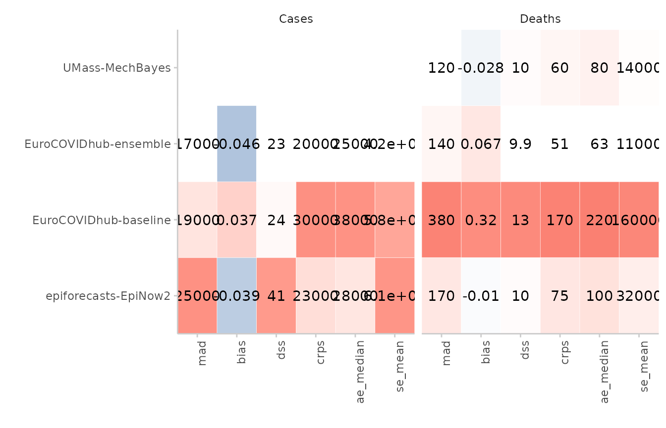
Score heatmap
We can also summarise one particular metric across different categories using a simple heatmap:
score(example_continuous) %>%
  summarise_scores(by = c("model", "location", "target_type")) %>%
  plot_heatmap(x = "location", metric = "bias") +
  facet_wrap(~ target_type)
#> The following messages were produced when checking inputs:
#> 1.  144 values for `prediction` are NA in the data provided and the corresponding rows were removed. This may indicate a problem if unexpected.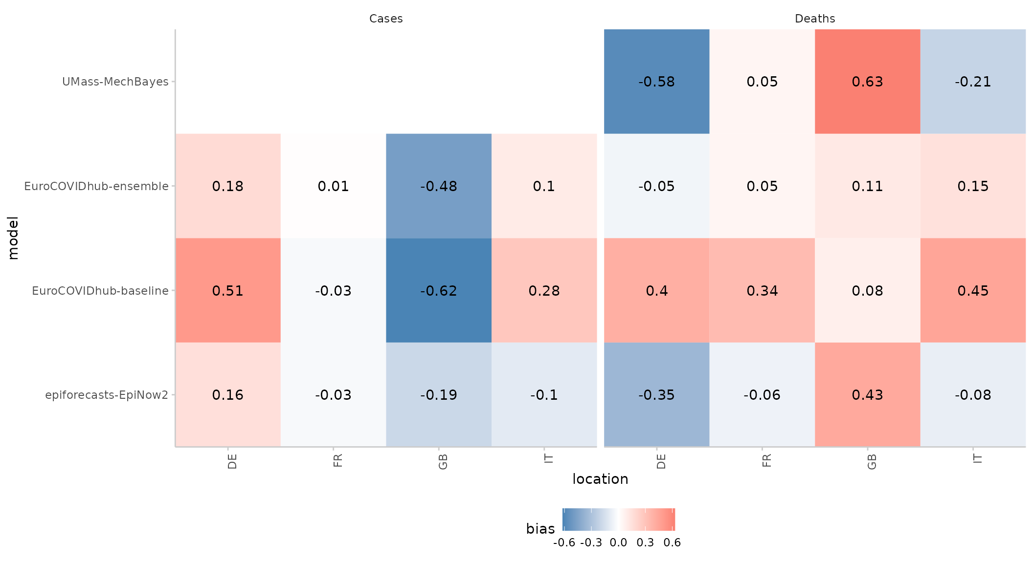
Weighted interval score components
The weighted interval score can be split up into three components: Over-prediction, under-prediction and dispersion. These can be visualised separately in the following way:
score(example_quantile) %>%
  summarise_scores(by = c("target_type", "model")) %>%
  plot_wis() +
  facet_wrap(~ target_type, scales = "free")
#> The following messages were produced when checking inputs:
#> 1.  144 values for `prediction` are NA in the data provided and the corresponding rows were removed. This may indicate a problem if unexpected.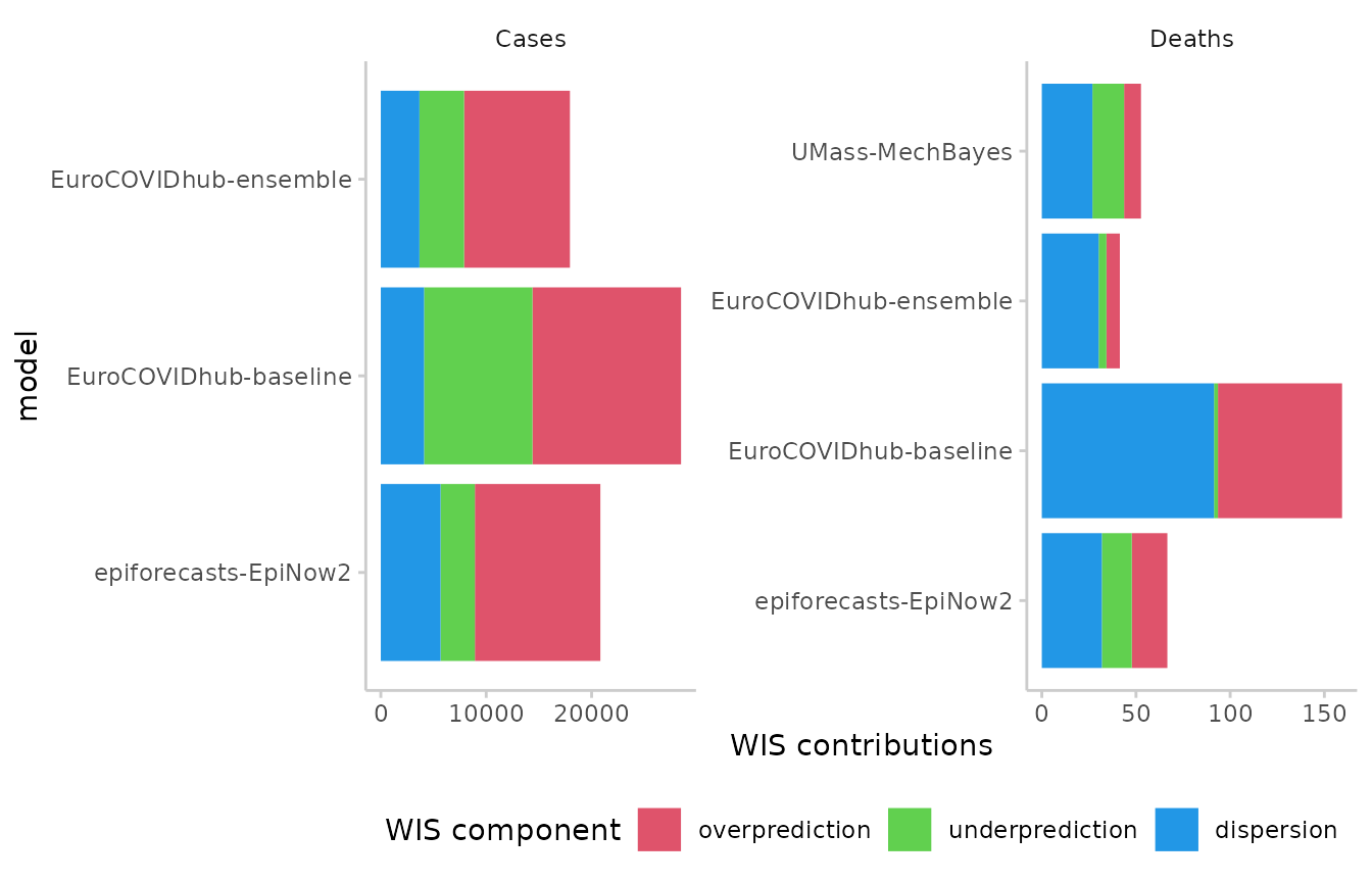
Calibration
Calibration is a measure statistical consistency between the forecasts and the observed values. The most common way of assessing calibration (more precisely: probabilistic calibration) are PIT histograms. The probability integral transform (PIT) is equal to the cumulative distribution function of a forecast evaluated at the true observed value. Ideally, pit values should be uniformly distributed after the transformation.
We can compute pit values as such:
example_continuous %>%
  pit(by = "model")
#> The following messages were produced when checking inputs:
#> 1.  144 values for `prediction` are NA in the data provided and the corresponding rows were removed. This may indicate a problem if unexpected.
#>                      model pit_value
#>   1: EuroCOVIDhub-baseline     0.025
#>   2: EuroCOVIDhub-baseline     0.525
#>   3: EuroCOVIDhub-baseline     0.000
#>   4: EuroCOVIDhub-baseline     0.000
#>   5: EuroCOVIDhub-baseline     0.200
#>  ---
#> 883:       UMass-MechBayes     0.950
#> 884:       UMass-MechBayes     0.500
#> 885:       UMass-MechBayes     0.100
#> 886:       UMass-MechBayes     0.450
#> 887:       UMass-MechBayes     0.100
And visualise the results as such:
example_continuous %>%
  pit(by = c("model", "target_type")) %>%
  plot_pit() +
  facet_grid(model ~ target_type)
#> The following messages were produced when checking inputs:
#> 1.  144 values for `prediction` are NA in the data provided and the corresponding rows were removed. This may indicate a problem if unexpected.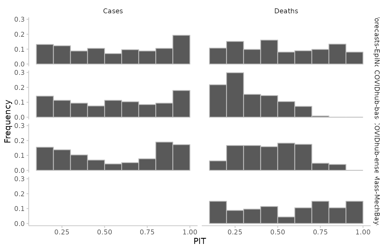
Similarly for quantile-based forecasts:
example_quantile[quantile %in% seq(0.1, 0.9, 0.1), ] %>%
  pit(by = c("model", "target_type")) %>%
  plot_pit() +
  facet_grid(model ~ target_type)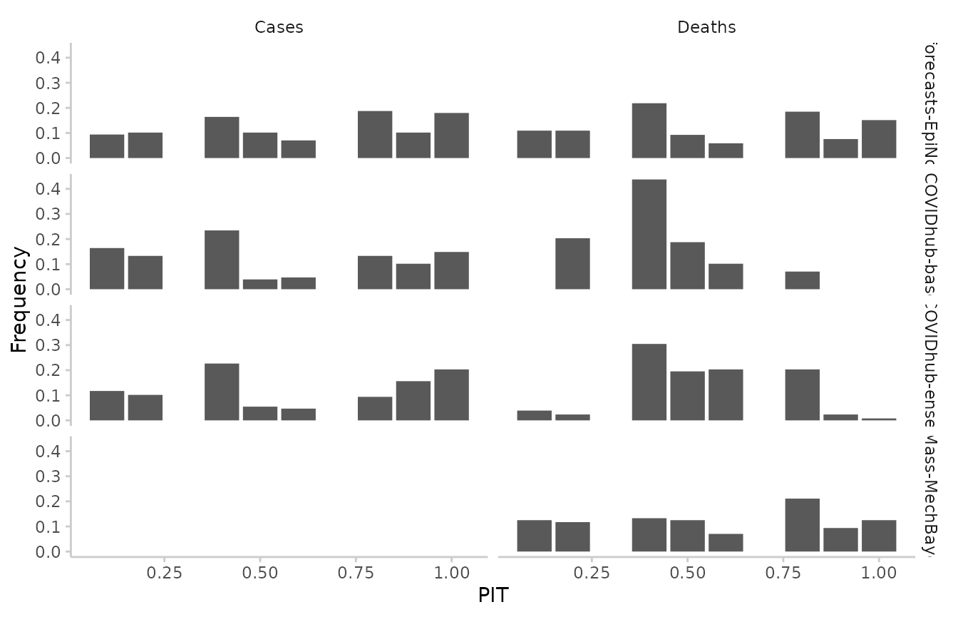
Another way to look at calibration are interval coverage and quantile coverage. Interval coverage is the percentage of true values that fall inside a given central prediction interval. Quantile coverage is the percentage of observed values that fall below a given quantile level.
In order to plot interval coverage, you need to include “range” in
the by argument to summarise_scores(). The
green area on the plot marks conservative behaviour, i.e. your empirical
coverage is greater than it nominally need be (e.g. 55% of true values
covered by all 50% central prediction intervals.)
example_quantile %>%
  score() %>%
  summarise_scores(by = c("model", "range")) %>%
  plot_interval_coverage()
#> The following messages were produced when checking inputs:
#> 1.  144 values for `prediction` are NA in the data provided and the corresponding rows were removed. This may indicate a problem if unexpected.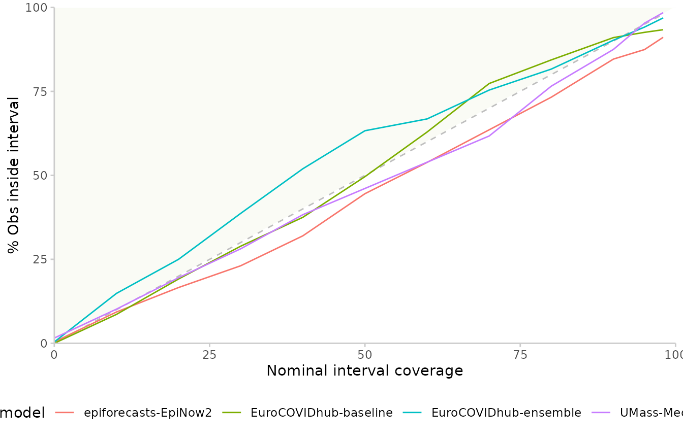
To visualise quantile coverage, you need to include “quantile” in
by. Again, the green area corresponds to conservative
forecasts, where central prediction intervals would cover more than
needed.
example_quantile %>%
  score() %>%
  summarise_scores(by = c("model", "quantile")) %>%
  plot_quantile_coverage()
#> The following messages were produced when checking inputs:
#> 1.  144 values for `prediction` are NA in the data provided and the corresponding rows were removed. This may indicate a problem if unexpected.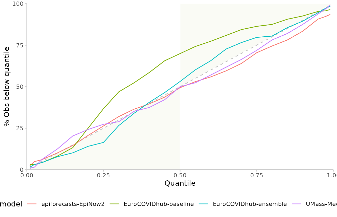
Pairwise comparisons
Relative scores for different models can be computed using pairwise comparisons, a sort of pairwise tournament where all combinations of two models are compared against each other based on the overlapping set of available forecasts common to both models. Internally, a ratio of the mean scores of both models is computed. The relative score of a model is then the geometric mean of all mean score ratios which involve that model. When a baseline is provided, then that baseline is excluded from the relative scores for individual models (which therefore differ slightly from relative scores without a baseline) and all relative scores are scaled by (i.e. divided by) the relative score of the baseline model.
In scoringutils, pairwise comparisons can be made in two
ways: Through the standalone function pairwise_comparison()
or from within summarise_scores() which simply adds
relative scores to an existing set of scores.
example_quantile %>%
  score() %>%
  pairwise_comparison(by = "model", baseline = "EuroCOVIDhub-baseline")
#> The following messages were produced when checking inputs:
#> 1.  144 values for `prediction` are NA in the data provided and the corresponding rows were removed. This may indicate a problem if unexpected.
#>                     model       compare_against mean_scores_ratio         pval
#>  1: EuroCOVIDhub-baseline  epiforecasts-EpiNow2         1.3703452 9.164893e-18
#>  2: EuroCOVIDhub-baseline EuroCOVIDhub-ensemble         1.5925819 2.608666e-32
#>  3: EuroCOVIDhub-baseline       UMass-MechBayes         3.0275019 2.627464e-20
#>  4: EuroCOVIDhub-baseline EuroCOVIDhub-baseline         1.0000000 1.000000e+00
#>  5: EuroCOVIDhub-ensemble       UMass-MechBayes         0.7867229 1.244731e-04
#>  6: EuroCOVIDhub-ensemble  epiforecasts-EpiNow2         0.8606607 1.881520e-02
#>  7: EuroCOVIDhub-ensemble EuroCOVIDhub-baseline         0.6279112 2.608666e-32
#>  8: EuroCOVIDhub-ensemble EuroCOVIDhub-ensemble         1.0000000 1.000000e+00
#>  9:       UMass-MechBayes EuroCOVIDhub-ensemble         1.2710955 1.244731e-04
#> 10:       UMass-MechBayes  epiforecasts-EpiNow2         0.7439673 7.253878e-03
#> 11:       UMass-MechBayes EuroCOVIDhub-baseline         0.3303053 2.627464e-20
#> 12:       UMass-MechBayes       UMass-MechBayes         1.0000000 1.000000e+00
#> 13:  epiforecasts-EpiNow2       UMass-MechBayes         1.3441452 7.253878e-03
#> 14:  epiforecasts-EpiNow2 EuroCOVIDhub-ensemble         1.1618981 1.881520e-02
#> 15:  epiforecasts-EpiNow2 EuroCOVIDhub-baseline         0.7297431 9.164893e-18
#> 16:  epiforecasts-EpiNow2  epiforecasts-EpiNow2         1.0000000 1.000000e+00
#>         adj_pval relative_skill scaled_rel_skill
#>  1: 3.665957e-17      1.6032604        1.0000000
#>  2: 1.565200e-31      1.6032604        1.0000000
#>  3: 1.313732e-19      1.6032604        1.0000000
#>  4: 1.000000e+00      1.6032604        1.0000000
#>  5: 3.734192e-04      0.8074916        0.5036559
#>  6: 1.881520e-02      0.8074916        0.5036559
#>  7: 1.565200e-31      0.8074916        0.5036559
#>  8: 1.000000e+00      0.8074916        0.5036559
#>  9: 3.734192e-04      0.7475873        0.4662919
#> 10: 1.450776e-02      0.7475873        0.4662919
#> 11: 1.313732e-19      0.7475873        0.4662919
#> 12: 1.000000e+00      0.7475873        0.4662919
#> 13: 1.450776e-02      1.0332277        0.6444541
#> 14: 1.881520e-02      1.0332277        0.6444541
#> 15: 3.665957e-17      1.0332277        0.6444541
#> 16: 1.000000e+00      1.0332277        0.6444541
example_quantile %>%
  score() %>%
  summarise_scores(
    by = "model", relative_skill = TRUE, baseline = "EuroCOVIDhub-baseline"
  )
#> The following messages were produced when checking inputs:
#> 1.  144 values for `prediction` are NA in the data provided and the corresponding rows were removed. This may indicate a problem if unexpected.
#>                    model interval_score dispersion underprediction
#> 1: EuroCOVIDhub-baseline    14321.48926 2096.95360      5143.53567
#> 2: EuroCOVIDhub-ensemble     8992.62316 1846.85278      2120.64029
#> 3:       UMass-MechBayes       52.65195   26.87239        16.80095
#> 4:  epiforecasts-EpiNow2    10827.40786 2950.73422      1697.23411
#>    overprediction coverage_deviation        bias   ae_median relative_skill
#> 1:    7081.000000         0.00201087  0.21851562 19353.42969      1.6032604
#> 2:    5025.130095         0.04871603  0.00812500 12077.10156      0.8074916
#> 3:       8.978601        -0.02312500 -0.02234375    78.47656      0.7475873
#> 4:    6179.439535        -0.05516986 -0.04336032 14521.10526      1.0332277
#>    scaled_rel_skill
#> 1:        1.0000000
#> 2:        0.5036559
#> 3:        0.4662919
#> 4:        0.6444541
If using the pairwise_comparison() function, we can also
visualise pairwise comparisons by showing the mean score ratios between
models. By default, smaller values are better and the model we care
about is showing on the y axis on the left, while the model against it
is compared is shown on the x-axis on the bottom. In the example above,
the EuroCOVIDhub-ensemble performs best (it only has values smaller 1),
while the EuroCOVIDhub-baseline performs worst (and only has values
larger than 1). For cases, the UMass-MechBayes model is of course
excluded as there are no case forecasts available and therefore the set
of overlapping forecasts is empty.
example_quantile %>%
  score() %>%
  pairwise_comparison(by = c("model", "target_type")) %>%
  plot_pairwise_comparison() +
  facet_wrap(~ target_type)
#> The following messages were produced when checking inputs:
#> 1.  144 values for `prediction` are NA in the data provided and the corresponding rows were removed. This may indicate a problem if unexpected.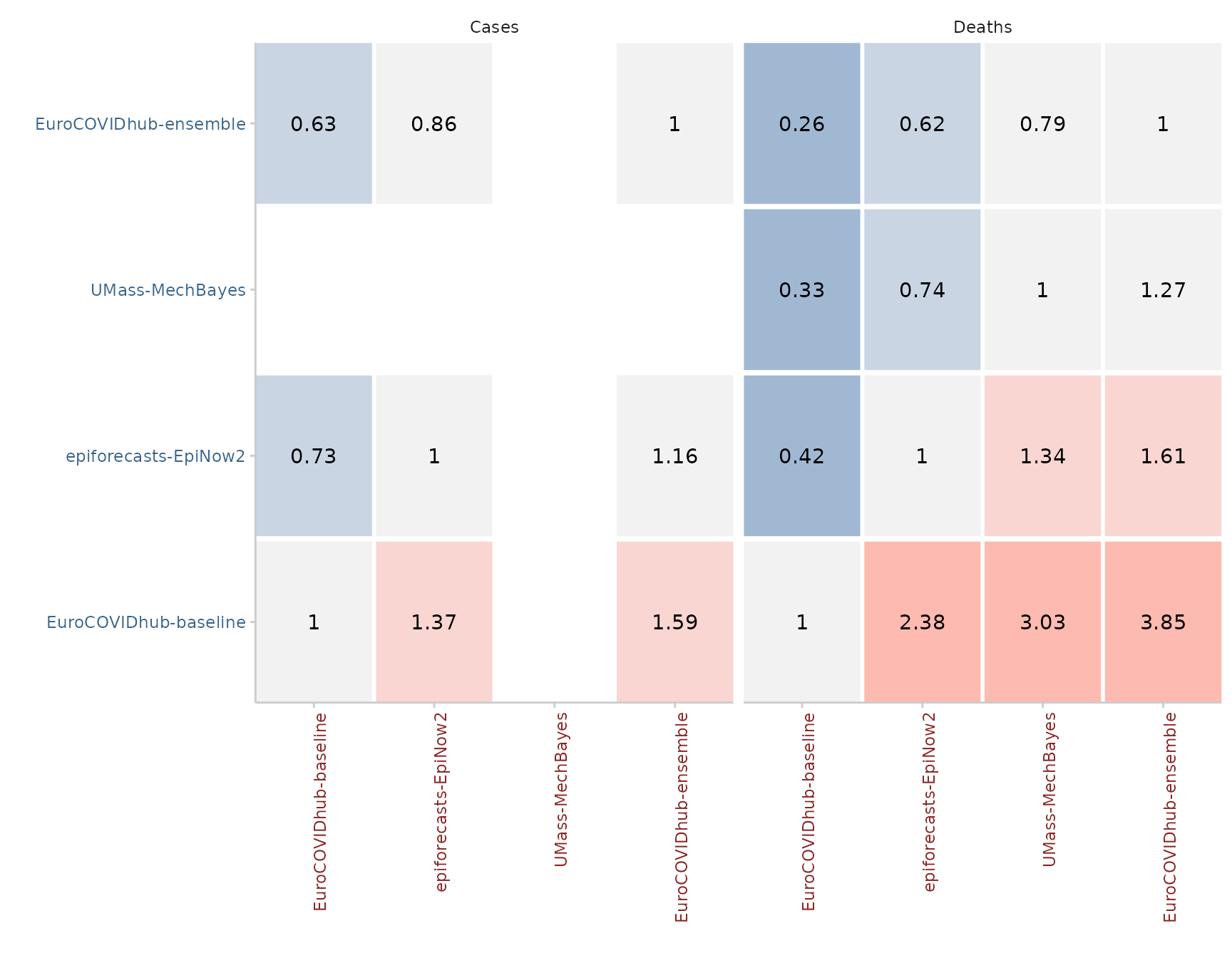
Additional analyses and visualisations
Correlation between scores
It may sometimes be interesting to see how different scores correlate
with each other. We can examine this using the function
correlation(). When dealing with quantile-based forecasts,
it is important to call summarise_scorees() before
correlation() to summarise over quantiles before computing
correlations.
example_quantile %>%
  score() %>%
  summarise_scores() %>%
  correlation()
#> The following messages were produced when checking inputs:
#> 1.  144 values for `prediction` are NA in the data provided and the corresponding rows were removed. This may indicate a problem if unexpected.
#>    interval_score dispersion underprediction overprediction coverage_deviation
#> 1:           1.00       0.46            0.28           0.94              -0.34
#> 2:           0.46       1.00            0.15           0.32              -0.12
#> 3:           0.28       0.15            1.00          -0.03              -0.33
#> 4:           0.94       0.32           -0.03           1.00              -0.25
#> 5:          -0.34      -0.12           -0.33          -0.25               1.00
#> 6:           0.11       0.11           -0.35           0.22               0.06
#> 7:           0.99       0.54            0.34           0.90              -0.38
#>     bias ae_median             metric
#> 1:  0.11      0.99     interval_score
#> 2:  0.11      0.54         dispersion
#> 3: -0.35      0.34    underprediction
#> 4:  0.22      0.90     overprediction
#> 5:  0.06     -0.38 coverage_deviation
#> 6:  1.00      0.10               bias
#> 7:  0.10      1.00          ae_median
Visualising correlations:
example_quantile %>%
  score() %>%
  summarise_scores() %>%
  correlation() %>%
  plot_correlation()
#> The following messages were produced when checking inputs:
#> 1.  144 values for `prediction` are NA in the data provided and the corresponding rows were removed. This may indicate a problem if unexpected.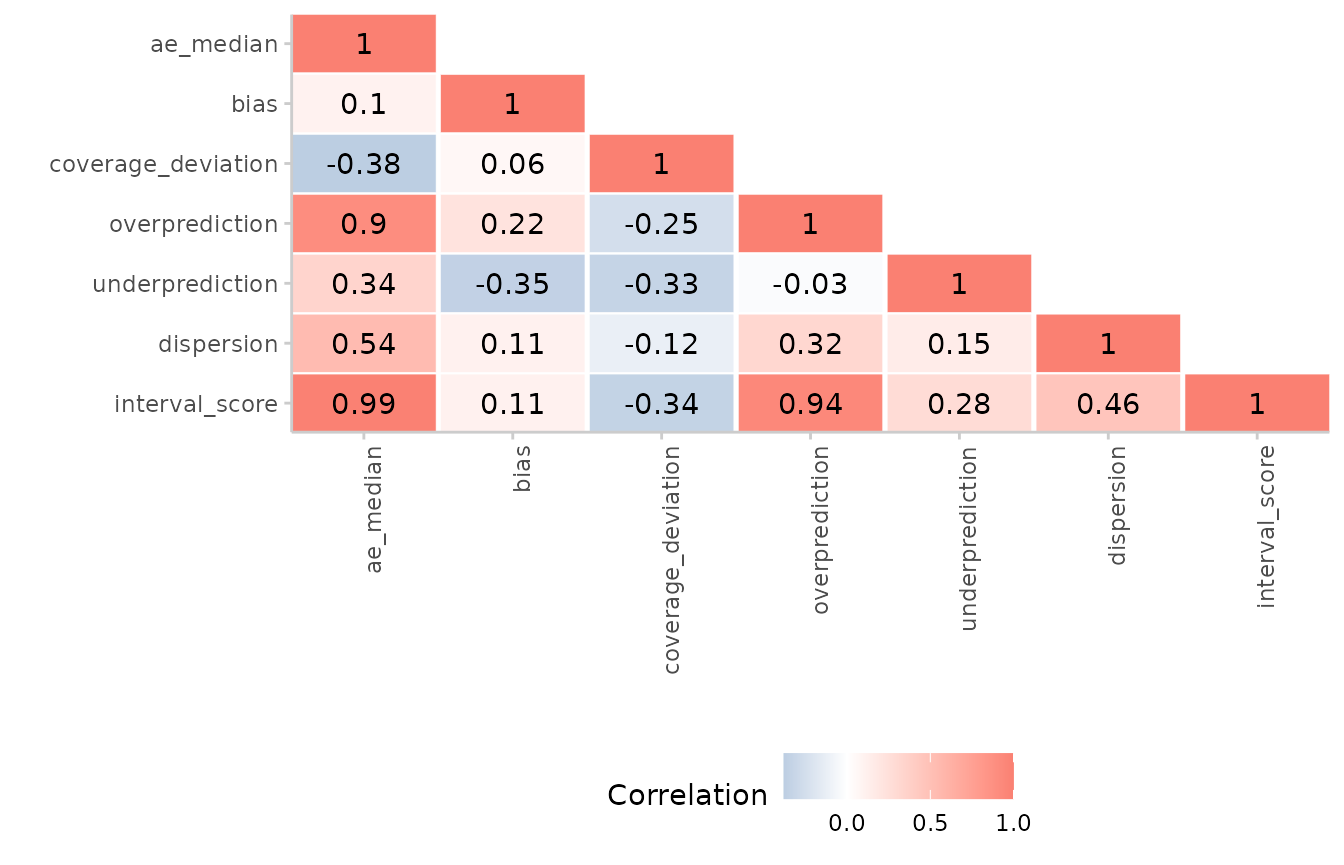
Scores by interval ranges
If you would like to see how different forecast interval ranges contribute to average scores, you can visualise scores by interval range:
example_quantile %>%
  score() %>%
  summarise_scores(by = c("model", "range", "target_type")) %>%
  plot_ranges() +
  facet_wrap(~ target_type, scales = "free")
#> The following messages were produced when checking inputs:
#> 1.  144 values for `prediction` are NA in the data provided and the corresponding rows were removed. This may indicate a problem if unexpected.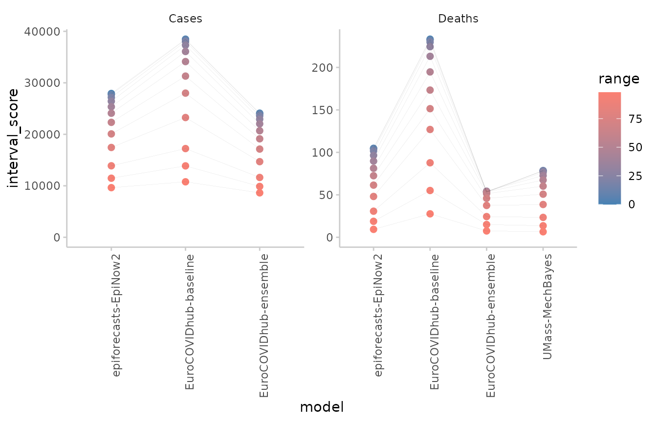
Converting to quantile-based forecasts
Different metrics are available for different forecasting formats. In some cases, you may for example have forecasts in a sample-based format, but wish to make use of some of the functionality only available to quantile-based forecasts. For example, you may want to use the decomposition of the weighted interval score, or may like to compute interval coverage values.
You can convert your sample-based forecasts into a quantile-based
format using the function sample_to_quantile(). There is,
however, one caveat: Quantiles will be calculated based on the
predictive samples, which may introduce a bias if the number of
available samples is small.
example_integer %>%
  sample_to_quantile(
    quantiles = c(0.01, 0.025, seq(0.05, 0.95, 0.05), 0.975, 0.99)
  ) %>%
  score() %>%
  add_coverage(by = c("model", "target_type"))
#> The following messages were produced when checking inputs:
#> 1.  3312 values for `prediction` are NA in the data provided and the corresponding rows were removed. This may indicate a problem if unexpected.
#>                        model target_type location location_name target_end_date
#>     1: EuroCOVIDhub-baseline       Cases       DE       Germany      2021-05-08
#>     2: EuroCOVIDhub-baseline       Cases       DE       Germany      2021-05-08
#>     3: EuroCOVIDhub-baseline       Cases       DE       Germany      2021-05-08
#>     4: EuroCOVIDhub-baseline       Cases       DE       Germany      2021-05-08
#>     5: EuroCOVIDhub-baseline       Cases       DE       Germany      2021-05-08
#>    ---
#> 20397:  epiforecasts-EpiNow2      Deaths       IT         Italy      2021-07-24
#> 20398:  epiforecasts-EpiNow2      Deaths       IT         Italy      2021-07-24
#> 20399:  epiforecasts-EpiNow2      Deaths       IT         Italy      2021-07-24
#> 20400:  epiforecasts-EpiNow2      Deaths       IT         Italy      2021-07-24
#> 20401:  epiforecasts-EpiNow2      Deaths       IT         Italy      2021-07-24
#>        forecast_date horizon range interval_score dispersion underprediction
#>     1:    2021-05-03       1     0    29379.00000    0.00000               0
#>     2:    2021-05-03       1    10    27857.47500 3012.07500               0
#>     3:    2021-05-03       1    10    27857.47500 3012.07500               0
#>     4:    2021-05-03       1    20    26443.96000 4109.76000               0
#>     5:    2021-05-03       1    20    26443.96000 4109.76000               0
#>    ---
#> 20397:    2021-07-12       2    90       21.21000   21.21000               0
#> 20398:    2021-07-12       2    95       15.00563   15.00563               0
#> 20399:    2021-07-12       2    95       15.00563   15.00563               0
#> 20400:    2021-07-12       2    98        6.28890    6.28890               0
#> 20401:    2021-07-12       2    98        6.28890    6.28890               0
#>        overprediction coverage coverage_deviation bias quantile ae_median
#>     1:        29379.0        0               0.00 0.98    0.500   29379.0
#>     2:        24845.4        0              -0.10 0.98    0.450   29379.0
#>     3:        24845.4        0              -0.10 0.98    0.550   29379.0
#>     4:        22334.2        0              -0.20 0.98    0.400   29379.0
#>     5:        22334.2        0              -0.20 0.98    0.600   29379.0
#>    ---
#> 20397:            0.0        1               0.10 0.70    0.950      73.5
#> 20398:            0.0        1               0.05 0.70    0.025      73.5
#> 20399:            0.0        1               0.05 0.70    0.975      73.5
#> 20400:            0.0        1               0.02 0.70    0.010      73.5
#> 20401:            0.0        1               0.02 0.70    0.990      73.5
#>        quantile_coverage coverage_50 coverage_90
#>     1:              TRUE   0.3828125   0.7265625
#>     2:              TRUE   0.3828125   0.7265625
#>     3:              TRUE   0.3828125   0.7265625
#>     4:              TRUE   0.3828125   0.7265625
#>     5:              TRUE   0.3828125   0.7265625
#>    ---
#> 20397:              TRUE   0.5462185   0.9243697
#> 20398:             FALSE   0.5462185   0.9243697
#> 20399:              TRUE   0.5462185   0.9243697
#> 20400:             FALSE   0.5462185   0.9243697
#> 20401:              TRUE   0.5462185   0.9243697
Available metrics
An overview of available metrics can be found in the
metrics data set that is included in the package.
metrics
#>                                           Metric               Name
#>  1:                               Absolute error           ae_point
#>  2:                               Absolute error          ae_median
#>  3:                                Squared error           se_point
#>  4:                                Squared error            se_mean
#>  5: (Continuous) ranked probability score (CRPS)               crps
#>  6:                                    Log score          log_score
#>  7:              (Weighted) interval score (WIS)     interval_score
#>  8:                 Dawid-Sebastiani score (DSS)                dss
#>  9:                             Brier score (BS)        brier_score
#> 10:                            Interval coverage           coverage
#> 11:                           Coverage deviation coverage_deviation
#> 12:                            Quantile coverage  quantile_coverage
#> 13:                                   Dispersion         dispersion
#> 14:       Median Absolute Deviation (Dispersion)                mad
#> 15:                      Under-, Over-prediction    underprediction
#> 16:                      Under-, Over-prediction     overprediction
#> 17:         Probability integral transform (PIT)               crps
#> 18:                                   Dispersion         dispersion
#> 19:                                         Bias               bias
#> 20:                             Mean score ratio  mean_scores_ratio
#> 21:                               Relative skill     relative_skill
#> 22:                        Scaled relative skill   scaled_rel_skill
#>                                           Metric               Name
#>                                   Functions Discrete Continuous Binary Quantile
#>  1: score(), ae_point()), ae_median_sample(        +          +      -        +
#>  2: score(), ae_point()), ae_median_sample(        +          +      -        +
#>  3:   score(), se_point(), se_mean_sample()        +          +      -        +
#>  4:   score(), se_point(), se_mean_sample()        +          +      -        +
#>  5:                       score(), ae_point        +          +      -        -
#>  6:   score(), logs_sample(), logs_binary()        -          +      +        -
#>  7:               score(), interval_score()        +          +      -        +
#>  8:                   score(), dss_sample()        +          +      -        -
#>  9:                  score(), brier_score()        -          -      +        -
#> 10:                                 score()        -          -      -        +
#> 11:                                 score()        -          -      -        +
#> 12:                                 score()        +          +      -        -
#> 13:               score(), interval_score()        -          -      -        +
#> 14:                   score(), mad_sample()        +          +      -        -
#> 15:               score(), interval_score()        -          -      -        +
#> 16:               score(), interval_score()        -          -      -        +
#> 17:                          score(), pit()        +          +      -        +
#> 18:               score(), interval_score()        -          -      -        +
#> 19: score(), bias_sample(), bias_quantile()        +          +      -        +
#> 20:                   pairwise_comparison()        ~          ~      ~        ~
#> 21:          score(), pairwise_comparison()        ~          ~      ~        ~
#> 22:          score(), pairwise_comparison()        ~          ~      ~        ~
#>                                   Functions Discrete Continuous Binary Quantile
#>                                                                                                                                                                                                           Info
#>  1:                                                                                                                                               Suitable for scoring the median of a predictive distribution
#>  2:                                                                                                                                               Suitable for scoring the median of a predictive distribution
#>  3:                                                                                                                                                Suitable for scoring the mean of a predictive distribution.
#>  4:                                                                                                                                                Suitable for scoring the mean of a predictive distribution.
#>  5:                           Proper scoring rule (smaller is better), takes entire predictive distribution into account (global), penalises over- and under-confidence similarly, stable handling of outliers
#>  6:                               Proper scoring rule, smaller is better, equals negative log of the predictive density at observed value (local), penalises over-confidence severely, susceptible to outliers
#>  7:                                                              Proper scoring rule, smaller is better, similar properties to CRPS and converges to CRPS for an increasing number of equally spaced intervals
#>  8:                           Proper scoring rule, smaller is better, evaluates forecast based on mean and sd of predictive distribution (global), susceptible to outliers, penalises over-confidence severely
#>  9:                                                                                    Proper scoring rule, smaller is better, equals CRPS for binary outcomes, penalises over- and under-confidence similarly
#> 10:                                                 Proportion of observations falling inside a given central prediction interval (= 'empirical interval coverage'). Used to assess probabilistic calibration.
#> 11:                                                                                               Average difference between empirical and nominal interval coverage (coverage that should have been realised)
#> 12:                                                                                         Proportion of observations below a given quantile of the predictive CDF. Used to assess probabilistic calibration.
#> 13:                                                                                                                                       Dispersion component of WIS, measures width of predictive intervals.
#> 14:                                                                                                                    Measure for dispersion of a forecast: median of the absolute deviations from the median
#> 15:                                                                                                                                            Absolute amount of over-or under-prediction (components of WIS)
#> 16:                                                                                                                                            Absolute amount of over-or under-prediction (components of WIS)
#> 17:                                                                                   PIT transform is the CDF of the predictive distribution evaluated at the observed values. PIT values should be uniform.
#> 18:                                                                                                                                       Dispersion component of WIS, measures width of predictive intervals.
#> 19:                                                                                       Measure of relative tendency to over- or under-predict (aspect of calibration), bounded between -1 and 1 (ideally 0)
#> 20:                                                                                                             Compares performance of two models. Properties depend on the metric chosen for the comparison.
#> 21:                                                         Ranks models based on pairwise comparisons, useful in the context of missing forecasts. Properties depend on the metric chosen for the comparison.
#> 22: Ranks models based on pairwise comparisons, useful in the context of missing forecasts. Scaled (i.e. divided) by the score of a baseline model. Properties depend on the metric chosen for the comparison.
#>                                                                                                                                                                                                           Info